Research Papers

A Two-Level Approach based on Integration of Bagging and Voting for Outlier Detection

  • Alican Dogan 1 ,
  • Derya Birant , 2,
Expand
  • 1The Graduate School of Natural and Applied Sciences, Dokuz Eylul University, Izmir, Turkey
  • 2Department of Computer Engineering, Dokuz Eylul University, Izmir, Turkey
Derya Birant (E-mail: )

Received date: 2019-12-13

  Request revised date: 2020-04-27

  Accepted date: 2020-04-29

  Online published: 2020-05-24

Copyright

Copyright reserved © 2020

Abstract

Purpose: The main aim of this study is to build a robust novel approach that is able to detect outliers in the datasets accurately. To serve this purpose, a novel approach is introduced to determine the likelihood of an object to be extremely different from the general behavior of the entire dataset.

Design/methodology/approach: This paper proposes a novel two-level approach based on the integration of bagging and voting techniques for anomaly detection problems. The proposed approach, named Bagged and Voted Local Outlier Detection (BV-LOF), benefits from the Local Outlier Factor (LOF) as the base algorithm and improves its detection rate by using ensemble methods.

Findings: Several experiments have been performed on ten benchmark outlier detection datasets to demonstrate the effectiveness of the BV-LOF method. According to the results, the BV-LOF approach significantly outperformed LOF on 9 datasets of 10 ones on average.

Research limitations: In the BV-LOF approach, the base algorithm is applied to each subset data multiple times with different neighborhood sizes (k) in each case and with different ensemble sizes (T). In our study, we have chosen k and T value ranges as [1-100]; however, these ranges can be changed according to the dataset handled and to the problem addressed.

Practical implications: The proposed method can be applied to the datasets from different domains (i.e. health, finance, manufacturing, etc.) without requiring any prior information. Since the BV-LOF method includes two-level ensemble operations, it may lead to more computational time than single-level ensemble methods; however, this drawback can be overcome by parallelization and by using a proper data structure such as R*-tree or KD-tree.

Originality/value: The proposed approach (BV-LOF) investigates multiple neighborhood sizes (k), which provides findings of instances with different local densities, and in this way, it provides more likelihood of outlier detection that LOF may neglect. It also brings many benefits such as easy implementation, improved capability, higher applicability, and interpretability.

Cite this article

Alican Dogan , Derya Birant . A Two-Level Approach based on Integration of Bagging and Voting for Outlier Detection[J]. Journal of Data and Information Science, 2020 , 5(2) : 111 -135 . DOI: 10.2478/jdis-2020-0014

1 Introduction

In recent years, various studies require data mining that can find outliers and protect system reliability. Outliers are observations that differ significantly from most of the samples in the dataset. They could be perceived as though they are generated by a different process. Generally, the number of outliers is comparably much less than the normal behaving data (typically lower than 10%). Data instances containing extreme feature values out of the accepted range may cause a negative effect on data analyses such as regression or may provide useful information about data such as terrorist attacks. Outlier analysis is especially adequate for fraud detection which is performed by an anomaly detection mechanism. Network intrusion detection, fraud detection in banking and telecommunications are some of the application areas of outlier detection (Tang & He, 2017).
If any data point is extremely different from the whole data in a process, then it is marked as an outlier (Qi & Chen, 2018). Outliers may emerge because of various causes such as malicious attacks, environmental factors, human errors, abnormal conditions, measurement errors, and hardware malfunction. Outlier detection is related but slightly different from novelty detection, which is concerned with the identification of new or unknown data not covered by the training data. Outlier detection makes the model adapt for normal behaving data, thus abnormally behaving data could be detected by the built model since it does not fit the conditioned model. Local Outlier Factor (LOF) and Isolation Forest (IF) are some of the soft computing methods dealing with this problem (Domingues et al., 2018).
However, it is not always straightforward to perform anomaly detection successfully for many methods (Cao et al., 2017). Sampling approaches are not generally used for this task since they are affected by over-sampling minority values or under-sampling majority values. Detecting an outlier in any context is a challenging task due to the lack of a known underlying model and the strong dependence of the existing methods on input parameters. In order to overcome these problems, in this study, we propose a new ensemble-based outlier detection approach, named Bagged and Voted Local Outlier Detection (BV-LOF). Our approach uses the LOF algorithm as a base detector on various subsets of data and aggregates the obtained results by a combining mechanism.
The main contributions of this paper are three-fold: (i) It proposes a novel approach (BV-LOF), which integrates two different styles of ensemble learning (bagging and voting) using the Local Outlier Factor (LOF) algorithm in order to detect outliers. In this way, it is aimed at improving the general performance of LOF on detecting anomalies. (ii) This is the first study that runs the LOF algorithm with different input parameter k values (the number of nearest neighbors) many times and incorporates them in a single solution. (iii) The proposed approach differs from the existing approaches since it does not neglect the changing effect of a distinct group of features chosen from the whole set of features.
In the experimental studies, ten benchmark outlier datasets were used and the results were compared with the ones obtained by using the LOF method. Area Under the Receiver Operating Characteristics Curve (AUC) measure was used to evaluate the outlier detection performance of the proposed method for all datasets. According to the experimental results, the proposed two-level approach (BV-LOF) demonstrated better performance compared to LOF.
The rest of this paper is organized as follows. Section 2 describes outlier detection studies that have been conducted by researchers so far. Section 3 explains the proposed method (BV-LOF) in detail with its benefits and time complexity. Section 4 presents the datasets used in the experiments and discusses the experimental results obtained by the comparison of two methods: LOF and BV-LOF. Final comments on the study and possible future works are presented in Section 5.

2 Related work

In the majority of the cases, the number of instances that belong to the class of outliers is less than 10% of the total number of instances in the whole training set (Wu et al., 2018). Their identification becomes one of the most challenging situations in data analysis, hence, in general, the probabilities of detecting an anomaly in a dataset are extremely low for many methods. The studies presented in the literature have shown that many traditional classification, clustering, and regression algorithms are not capable of dealing with outliers. The reason behind this situation is that learning algorithms are likely to misinterpret the data containing outliers. For this reason, the proposed approach in this paper can be applied as a separate data preprocessing step before classification, regression, and clustering tasks.
In the literature, many different outlier detection algorithms have been proposed to observe the presence of outliers effectively. A group of algorithms uses the reconstruction error to find contaminations (Balamurali & Melkumvan, 2018), in which the data that have greater reconstruction errors are labeled as outliers. These algorithms assume that strong statistical correlations exist among the attributes of normally behaving data. These reconstruction-based techniques can capture the correlations by reducing the reconstruction errors of data having the expected behavior. For this reason, the outliers have comparatively larger reconstruction errors than normal data.
Different assumptions have been made by the existing outlier detection approaches. These assumptions vary and make all the approaches differ from each other. Density-based and distance-based techniques are generally the source of most of the complex algorithms (Lopes et al., 2018).
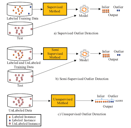
As shown in Figure 1, the learning scenarios proposed by the current outlier detection methods can be grouped into three categories: supervised, semi-supervised, and unsupervised. In supervised outlier detection, class-labeled data tagged as inlier and outlier is provided for training. So, distinct classes of data are available like in binary or multi-class classification (Huang et al., 2012). Semi-supervised outlier detection can utilize labeled instances for only inlier class or can use both labeled data (tagged as inlier and outlier) and unlabeled data (maybe or may not be an outlier). In unsupervised outlier detection, the algorithm tries to learn from only unlabeled data (Pasillas-Diaz & Ratte, 2017), so it has no information about class labels. In this study, we proposed a novel outlier detection approach that focuses on unsupervised learning, so only data without label or class exist.
Unsupervised outlier detection approaches have also sub-categories: clustering-based, density-based, and relative density-based methods.
First, clustering-based techniques have the strategy that each instance either belongs to a cluster or not (called as an outlier). In these types of algorithms, data is split into clusters, and being a member of a cluster determines whether the instance is an anomaly or not. A binary decision is taken by the model. Therefore, it does not provide an extensive comprehension of the identified outliers.
Secondly, density-based techniques identify instances found in the areas with low density and named them as anomalies. An anomaly score is given to each instance based on the nearest neighbor (NN) distance strategy. Different density-based outlier detection methods have been proposed by researchers so far. Local Outlier Factor (LOF) is one of the most popular density-based methods that use NN methodology. For this reason, in this study, we preferred to use the LOF method because of its advantages such as being an unsupervised algorithm, easy to understand and implement, dealing with high dimensional data, and requiring no assumption of the underlying data.
Thirdly, in relative density-based techniques, anomalies are defined as observations that have lower relative density than its neighbors (Bandaragoda et al., 2017). This technique is proposed since the global density function causes the problem of limited identified local outliers in dense areas having low relative density to its neighbors. The ratio of density between an instance and its neighborhood is taken as a measure of relative density. In this way, instances with low density are labeled as outliers.
Figure 1. Learning scenarios for outlier detection models.
Several variants of the LOF algorithm have been implemented in order to overcome a disadvantage that the researchers observed in the original LOF. For example, Qin et al. (2019) proposed Weighted LOF (WLOF) to deal with the impact of data duplication. Gan and Zhou (2018) proposed the D-LOF approach, which uses the DBSCAN algorithm to optimize the LOF algorithm by dynamically adjusting the parameter k of the algorithm. Bhatt, Sharma and Ram (2013) proposed Modified LOF (MLOF), which also considers mean distance (m-distance) between an object and its k-distance neighborhood to enhance the performance of the LOF algorithm. In this paper, we proposed a novel approach, called BV-LOF, based on the LOF algorithm to improve its detection performance.
Ensemble learning is a supported mechanism in outlier detection tasks. Ensemble-based models utilize an outlier detection algorithm or a series of different algorithms more than once on various settings of the same dataset and combine the outputs to get the final anomaly score (Chakraborty, Narayanan, & Ghosh, 2019; Zhang et al., 2019). In the literature, several studies have been performed by using an ensemble strategy for this purpose (Chen et al., 2018; Hu et al., 2019; Li, Fang, & Yan, 2019; Wang & Mao, 2019). The previous studies have proven that ensemble learning yields advantages in many different applications such as process monitoring (Wang & Mao, 2019), video anomaly detection (Hu et al. 2019), maintenance prediction (Li, Fang & Yan, 2019) and image-based outlier detection (Chen et al., 2018). This is because, they try to minimize errors of judgment made by different models or differently selected subsets of data (Kaneko, 2018).
Lazarevic and Kumar (2005) proposed a feature bagging mechanism to create different datasets with randomly selected attributes before applying LOF on those datasets. However, k value selection can highly affect the detection performance of the algorithm. In the Bagged LOF approach, there is no information about k value (the number of nearest neighbors) selection and so input parameter k is chosen arbitrarily. Our approach solves this problem by considering multiple k values.
Differently from the previous studies, our approach consists of two consecutive phases: Bagging and Voting. In the first phase, differently chosen subsets of attributes are used to benefit from various correlations of input features. In the second stage, the effects of diverse k value selections are taken into consideration and their results are combined with a majority voting mechanism. In this way, the LOF method, which is easily affected by the input parameter, is made more robust for datasets.

3 Materials and method

3.1 Outlier detection problem

Let D be a dataset, denoted by D = {X1, X2, ..., Xn} with n tuples and d features, where each Xi refers to a d-dimensional vector, i.e. Xi = {xi1, xi2, ..., xid}, where xij is the value of the jth feature of xi and i = 1, 2, ..., n. So each record is a point in the d-dimensional feature space. Let F = {F1, F2, F3, ..., Fd} be the set of features, where xij Fj. Formally, an outlier detector for D is a d-dimensional function f(x1, x2, ..., xd). The output value of the function f at a specific point x = {x1, x2, ..., xd} of the d-dimensional feature space estimates the probability of the point to be an outlier. A data point pi is defined as an outlier with respect to function f if it is in some way “significantly different” from its neighbors.

3.2 Local outlier factor

Local Outlier Factor (LOF) method is aimed at finding extreme data points with the help of local deviation with respect to k number of instances in the neighborhood of a given instance (Breunig et al., 2000). Local density estimation can vary by using different types of distance measurement techniques. The locality is determined by k nearest neighbors. The local density of a selected instance is compared to the local densities of the samples in its neighborhood. The samples having comparably much lower local density than its nearest neighbors are assigned as outliers. In addition, the reachability distance concept is defined to get more stable results within clusters, which is the distance between two data points if the distance is greater than the distance between the sample and its kth neighbor. Otherwise, the reachability distance is assigned with the distance between the sample and its kth neighbor. At the end of the method, the LOF score is calculated which is expected to be a value of about 1. If this score is highly greater than 1, then the given data point is a possible candidate to be an outlier.
Definition 1. k-distance of a data point p
Given a dataset D and a positive number k, the k-distance (p) is defined as the distance d(p,o) between a data point p and an object o D such that
- for at least k objects o’ ∈ D-{p}, satisfying d(p,o’) ≤ d(p,o).
- for at most k-1 objects o’ ∈ D-{p}, satisfying d(p,o’) < d(p,o).
Definition 2. k-distance neighborhood of a data point p
Given a data point p of a dataset D and a positive number k, the k-distance neighborhood of p, named Nk(p), includes every item whose distance from p is not greater than the k-distance(p).
Nk(p) = { qD -{p} | d(p,q) ≤ k-distance(p) }
where any such object q is called a k-distance neighbor of p.
Definition 3. Reachability distance (reach-dist) of a data point p w.r.t. another data point o
For a positive number k, reach-dist is defined as the maximum distance of k-distance of the point o and the distance between two points p and o.
reach-distk(p,o) = max{k-distance(o), d(p,o)}
where d(p,o) is computed using a distance measure such as Euclidean or Manhattan distance.
Definition 4. Local reachability density (lrd) of a data point p
Given a dataset D, the local reachability density for a point pD is computed by the inverse of the average reach-dist based on the k-nearest neighbors Nk of p as given in Equation 3.
where |Nk(p)| is the number of the k-distance neighbors of p.
Definition 5. Local outlier factor (LOF) of a data point p
The LOF is a score assigned to each data point, which gives information about how likely the data point to be an outlier.

3.3 Proposed approach (BV-LOF)

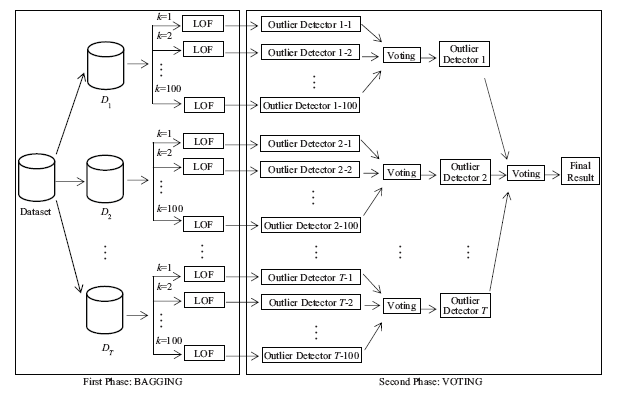
In this paper, we propose a novel two-level outlier detection approach, named Bagged and Voted Local Outlier Detection (BV-LOF). As shown in Figure 2, the BV-LOF approach has two main phases which are bagging and voting. Bagging, which is the short form of bootstrap aggregation, finds the outlier scores in a series of T iteration. At each iteration, it calculates the scores using a different feature set and a different size of the neighborhood (k). The voting stage of the approach combines the outputs of the outlier models by majority voting to determine the final result.
The BV-LOF approach provides a solution to improve the performance of the LOF algorithm. The intuition behind this approach is that the combination of diverse feature subsets and multiple variants of the same algorithm can supplement each other and collective decision provides an improvement on the overall detection rate. The integration of partial features provides many advantages over the full features that can be summarized as follows:
(1) Improving accuracy: Integration of partial features increases the possibility of selecting the right subset to improve the accuracy of the model. Since initially it is unknown that which subset of features is more adequate for outlier detection, creating different subsets with different sizes from full features and combining their decisions would be an effective strategy. In the previous studies (Aggarwal, 2017; Lazarevic & Kumar, 2005), it has also been proven that the performance of outlier detection can be significantly improved by using multiple feature subsets.
(2) Dealing with noisy data: Feature subset selection places a significant role in improving the performance of outlier detection, especially in the case of noisy data. When analyzing full features, the data becomes sparse, and the actual outliers become masked by the noise effects of high dimensions (Aggarwal, 2017). On the other hand, some deviations in a small feature subset may be significant enough to be indicative of abnormal behavior.
(3) Increasing robustness: In distance computation, the presence of irrelevant features can significantly degrade the performance of outlier detection (Lazarevic & Kumar, 2005). This is because all dimensions are weighted equally, even the irrelevant and unimportant dimensions. Since the outliers are often embedded in locally relevant subspaces, a set of feature subspaces can be sampled in order to improve robustness (Leng & Huang, 2011).
(4) Taking the advantages of ensemble learning: The advantages of the ensemble-based combined score of a given data point are very significant in the context of outlier detection (Aggarwal, 2017). The outlier scores obtained from different feature subspaces may be very different; therefore, it is usually difficult to fully trust the score of a single subspace, and so the combination of scores is crucial. In this sense, this approach is similar to that of taking advantage of the power of many weak learners to create a single strong learner in ensemble-based classification problems.
Figure 2. The general structure of the proposed BV-LOF approach.
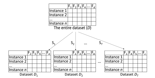
Figure 3 illustrates the feature bagging operation performed in the first phase of the BV-LOF approach. Let D be a dataset with d features and F={F1, F2, F3, ..., Fd} be the set of features, the feature subsets S = {S1, S2, S3, ..., ST} are generated by randomly selecting features (without replacement) from F, where T is the number of iterations (in other words ensemble size) and Si is a set of attributes with random size between d/2 and d-1, where i = {1,2,3,...,T}. For instance, in the example given in Figure 3, the features {F2, F5, F6, ..., Fa} are randomly selected without replacement for the first subset S1. To be more precise, the lower limit for the size is half of the number of features and the upper limit is the number of all features except for randomly selected one.
Figure 3. Feature subset selection operation in the first stage of the BV-LOF approach.
In the first step of the BV-LOF approach, the LOF algorithm is applied to each subset data multiple times with different sizes of the neighborhood (k) in each case. In our study, we chose k value range as [1-100] since in some previous studies (Alshawabkeh, Jang B, & Kaeli, 2010; Goldstein & Uchida, 2016) different k values between 1 and 100 were evaluated. This range is valid if the dataset has much more than 100 observations. In total, the LOF method is run T x 100 times. After that, an intermediate result is determined by combining the results of the different iterations of LOF with different k parameters (for k = 1,2,3,...,100) on the same feature subspace of the original dataset D using majority voting mechanism. In this way,T intermediate results are obtained. Lastly, these intermediate results are combined with another majority voting operation to determine the final result. If the majority of the subsets mark an instance as an outlier, then it is assigned as an extreme sample by the algorithm.
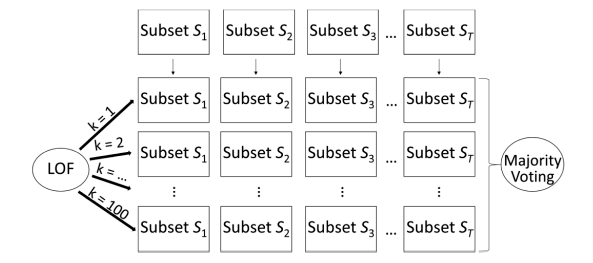
Figure 4 shows the majority voting operation of the BV-LOF approach. The LOF algorithm produces an output for each different size of the neighborhood (k) for each subset. An instance is scored by all the ensemble members; then these scores are combined to obtain an overall score for this instance. The main advantages of the proposed two-level ensemble model are: (i) it can reflect the effects of a different group of features which are neglected in the basic approach, and (ii) distinct kinds of k values may provide possible improvements on the results.
Figure 4. LOF application and majority voting operation in the second stage of the BV-LOF approach
The pseudo-code of the BV-LOF approach is presented in Algorithm 1. For each ensemble iteration, the size of the feature subset (R) is determined randomly in the range between d/2 and d-1 as proposed by Lazarevic & Kumar (2005), where d is the dimension of the dataset. After that, a set of features Si with size R is selected without replacement and these features are used to produce a lower-dimensional representation Di of the dataset D. The resulting data representation Di has a lower dimensionality, but it has the same number of instances as the original dataset D. BV-LOF feeds the LOF algorithm with different data representations Di for each iteration of the ensemble. The LOF algorithm is run 100 times with different size of neighborhood (k) parameter settings (from 1 to 100 by an increment of 1). The LOF algorithm returns a vector having labels for all the instances in the dataset. Totally, 100 output vectors are generated with respect to 100 different k values. After that, these vectors are combined by an inner majority voting mechanism to produce a result set with a unique label for each instance. The instances that are considered as outliers by LOF are marked with -1 and the inliers are labeled as 1. If the majority of the output vectors mark an instance as outlier then it is assigned as an outlier for the corresponding subset. Otherwise, the result of the inner ensemble becomes 1, which indicates that this instance is an inlier. After all the subsets (totally T subsets) have their own ensemble output vectors, outer majority voting is applied to get a final output vector in the same way.

3.4 An example of BV-LOF

In this section, the proposed approach (BV-LOF) is illustrated with an example. Assume that three feature subsets (S1, S2, and S3) are selected from all features in the original dataset D such as S1={F2,F5,F6,F8}, S2={F1,F3,F6, F7,F8} and S3={F1,F2,F4,F5,F7,F8}. After that, S1, S2, and S3 are used to generate sub-datasets D1, D2, and D3 from the original dataset D, respectively. In the example scenario, there are five instances and the input parameter k is set from 1 to 3 at each iteration. Sample LOF results obtained for each instance for each k value is given in Table 1. Firstly, majority voting result vectors (V1, V2, and V3) are obtained from the values returned from the LOF algorithm running with different k values (from 1 to 3). Inner majority voting mechanism is performed such that, for a data subset Di, if more than half of the result vectors marks the specific instance (Xi) as an outlier, then this instance is assigned as an outlier for that data subset. After all, inner voting results obtained for each data subset are re-combined by the outer majority voting scheme to find the ultimate result vector.
Table 1 An example to illustrate bagging and voting steps of BV-LOF approach.
D1 k=1 k=2 k=3 Voting
(V1)
D2 k=1 k=2 k=3 Voting
(V2)
D3 k=1 k=2 k=3 Voting
(V3)
V1 V2 V3 Voting
X1 1 1 1 1 X1 1 1 -1 1 X1 1 1 1 1 X1 1 1 1 1
X2 -1 -1 1 -1 X2 -1 -1 -1 -1 X2 1 -1 -1 -1 X2 -1 -1 -1 -1
X3 1 -1 1 1 X3 1 1 1 1 X3 1 1 -1 1 X3 1 1 1 1
X4 1 1 1 1 X4 1 1 1 1 X4 1 1 1 1 X4 1 1 1 1
X5 1 1 -1 1 X5 1 -1 -1 -1 X5 -1 -1 -1 -1 X5 1 -1 -1 -1

3.5 Advantages and disadvantages of the proposed approach (BV-LOF)

The main advantages of the proposed approach (BV-LOF) over other outlier detection methods can be summarized as follows:
• Detection of meaningful local outliers: It provides detection of local abnormally behaving data points with respect to the density of their neighboring data instances, instead of the global model.
• Running without any parameter for the neighborhood: It does not require the selection of k input parameter (the number of neighbors) which highly affects the performance of outlier detection.
• Applicability: Since it considers local densities of instances, it is proper for arbitrarily shaped data with groups of varying sizes, characteristics, and densities. Moreover, it has the ability to learn the underlying structure of data without any prior knowledge, i.e. without any assumption about the distributions of data points. In addition, it is independent of the domain of application, so it can be easily generalized for different problems such as network intrusion detection, fraud discovery in telecommunication, failure detection in manufacturing, email spam filtering, and medical data analysis. Furthermore, the BV-LOF algorithm is also suitable for high-dimensional data since it applies a feature selection scheme in the first stage of the algorithm.
• Providing ensemble-based outlier detection: The capability of outlier detection of the LOF method is improved using two-level ensemble approached which are bagging and voting.
• Parallelization: Although the BV-LOF algorithm runs more slowly than LOF since it operates on multiple data subsets and for multiple k values, the effect of this bottleneck could be decreased by executing the algorithm in a parallel way with multiple threads.
• Improved capability: The integration of various models generated by using different k values enables the algorithm to search for data points with various local densities and this increases the possibility of finding outliers that LOF may not detect.
• Easy implementation: It can be easily implemented since it does require any change in the general structure of the LOF algorithm.
• Interpretability: Output of the algorithm, which is in the form of observation score, can be easily interpreted by the user.
Besides the advantages of the BV-LOF approach, there are some drawbacks that can be summarized as follows:
• Performance depending on the k value range: Since the majority voting treats all LOF implementations with each k value equally, it may neglect the improvements obtained by few implementations with some k values if their decisions are surpassed by the majority.
• Computational cost: The BV-LOF method is slower than LOF because it requires multiple implementations for different subsets.
• Problem specific outliers: The meaning of an outlier may change according to the context of the data and the model does not provide any prior information about the significance of the outlier with respect to the usage criteria.

3.6 Time complexity of BV-LOF

In this section, the two-level proposed model is analyzed with respect to time complexity. The time complexity of the BV-LOF approach mainly depends on the time complexity of the base algorithm (LOF) and the ensemble size (in other words the number of iterations). More specifically, it depends on following parameters: the number of instances (n), the number of attributes (d), the selected feature size for subsets (between d/2 and d-1), the number of iterations (T) (ensemble size) and the range related to the input parameter (k). The first stage copies the values from the original dataset to the related subsets. In the average case, feature size becomes 3d/4 and the process takes O(T x n x 3d/4), which is in the order of n since it is much larger than the other terms. The second stage runs the LOF algorithm k times (i.e. 100 in this study) for each subset and, in the average case, it becomes k/2; so this process increases the time complexity by T x k x O(LOF(k/2)). While the time complexity of the inner voting operation is O(n x k), it is O(n x T) for outer voting operation.
The time complexity of LOF is near-quadratic with respect to the number of instances. However, different variations of LOF were proposed in the literature to reduce the time complexity of LOF such as IF-LOF (Cheng, Zou, & Dong, 2019), N2DLOF (Su et al., 2017), Top-n LOF (TOLF) (Yan, Cao, & Rundensteiner, 2017), BLOF (Bounded LOF) (Tang & Ngan, 2016), SimLOF (Sun et al., 2015), GridLOF (Wang & Huang, 2007), iLOF (Incremental LOF) (Pokrajac, Lazarevic, & Latecki, 2007), and MiLOF (memory efficient incremental local outlier) (Salehi et al., 2016). Therefore, instead of the traditional LOF algorithm, one of its variations can be used in the BV-LOF approach. The most computationally expensive step in BV-LOF is the k nearest neighbor search. To reduce the time complexity of BV-LOF, it is also possible to use various data structures such as R*-tree, KD-tree, Cover tree, and M-tree thanks to efficient nearest neighbor search.
Even though the running time of the BV-LOF method seems higher than the LOF algorithm due to the two-level ensemble operations such as divisions and integrations, this duration can be decreased by parallelization. If each subset is run simultaneously using different threads or processors, the negative effect of the proposed approach can be eliminated, and almost only LOF implementation and voting operations determine the length of the process.

4 Experimental studies

In this study, the BV-LOF method was implemented by using Scikit-Learn open-source library with Python programming language. We preferred Scikit-Learn since it provides many advantages such as ease of use, consistent and reliable API’s, a wide range of alternative algorithms, automatic hyperparameter tuning, integration of parallelization, and good documentation/tutorials. The LOF algorithm was selected to be used as a base outlier detection method. In all experiments, the default parameters of the algorithms in the Scikit-Learn library were used; expect k value and contamination parameter. After we had tested many different values of contamination parameters between 0.1 and 0.5, we concluded that the value of 0.22 produced better average results than the others. For this reason, we set this parameter as 0.22 in all the experiments. The values of the instances normalized using the preprocessing function of the Scikit-Learn library.
In order to validate the LOF and BV-LOF results, we used an external validation technique. External evaluation measure, which has been extensively studied for clustering and outlier detection tasks to examine the results, uses class labels known as ground truth. Since our study concentrates on datasets with class labels, it uses an external validity measure. Only the data, without class-labels, is used as input to the algorithm; however, the measure evaluates the goodness of the results with respect to class labels tagged as inlier and outlier. The measure evaluates the extent to which the structure discovered by an outlier detection algorithm matches by the externally given class labels. Since the external evaluation measure utilizes the true class labels in the comparison, it is a robust indicator of the true error rate of an outlier detection algorithm. By this way, external measure performs well in predicting the outlier detection errors.
When the data is imbalanced, using overall accuracy measure does not give sufficient information about the performance of the methods. Even though precision and recall scores can also be used, one of the most widely used validation measures in the research studies is the AUC (Area under the Receiver Operating Characteristics Curve) score. Thus, in the experimental studies, we used AUC validation measure to compare the performances of LOF and BV-LOF. The ROC curve is drawn by putting True Positive Rate (TPR) on the y-axis and False Positive Rate (FPR) on the x-axis. ROC Curve demonstrates how TPR changes according to FPR. AUC gives information about the degree of separability. That is to say, it reveals how successfully outliers are separated from the inliers by the applied model. Whenever the AUC ratio gets higher, the model detects outliers better. The AUC can be 1 at most and it means that the model is capable of detecting all the outliers and inliers without any error. Its value is in the range of [0, 1]. The AUC value 0.5 means that the model cannot differentiate outliers from normally behaving data well. When AUC is near 0.8, then the probability of the model to distinguish outliers from inliers is 80%. When this value becomes 0, it should be perceived that the model labels all the outliers as inliers and vice versa.

4.1 Dataset description

The proposed method BV-LOF has been tested with 10 outlier detection datasets ranging from 129 to 286,048 instances and from 6 to 41 attributes. The datasets are obtained from different domains. They are publicly available on well-known data repositories such as UCI Machine Learning Repository and Kaggle. They are frequently used for validating outlier (anomaly) detection algorithms in the literature (Reif, Goldstein, & Stahl, 2008; Yao et al., 2018; Zhou et al., 2013). Actually, these datasets are multi-class datasets having class labels. Here, the minority class (or classes) is considered as outliers compared to other larger classes. Hence, the instances in the smallest class(es) are marked as outliers, while all other instances are inliers. The overview of the datasets is given in Table 2. Generally, the density of the extreme samples is less than 10% of the entire dataset as is expected. The CoverType dataset is much larger than the rest with 286,048 records.
Table 2 Basic characteristics of the datasets.
ID Dataset # Instance # Feature % Outliers
1 CoverType 286,048 10 0.9
2 Glass 214 9 4.2
3 KDDCup 60,632 41 0.4
4 Lymphography 148 18 4.1
5 PageBlocks 5,473 10 10.2
6 PenDigits 9,868 16 0.2
7 Shuttle 1013 9 1.2
8 Stamps 340 9 9.1
9 Thyroid 3,772 6 2.5
10 Wine 129 13 7.7

4.2 Experimental results

In the experimental studies, the LOF algorithm was applied 100 times with different k values, where k changes from 1 to 100, and the AUC ratios were recorded. Moreover, the BV-LOF algorithm is run on the same dataset 100 times with different ensemble sizes (T), for T = 1,2,3,...,100, and their results were also noted. Finally, all the experimental results were compared for each dataset separately.
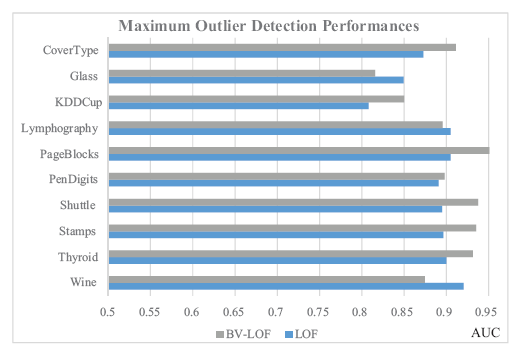
Figure 5 presents the comparison of the performance of LOF and BV-LOF methods in terms of maximum AUC values obtained in all trials. According to the results, the BV-LOF approach wins against LOF on 7 datasets of 10 ones. Thus, it is clearly seen that BV-LOF generally outperforms LOF on the datasets. For instance, BV-LOF produced a notable increment (~4%) in AUC for the Shuttle dataset. BV-LOF achieved the best performance with 83.92% AUC for the PageBlocks dataset. However, it was not able to get better results for Glass, Lymphography, and Wine datasets. In those datasets, different k values producing max performance are so limited and there is a great difference in AUC scores obtained from the best k values and the other values. This situation causes majority voting operation to smooth the effect of best k values by considering all k equally.
Figure 5. Comparison between LOF and BV-LOF methods in terms of maximum AUC values.
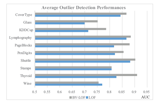
Figure 6 shows the comparative results of LOF and BV-LOF in terms of average AUC scores. Apparently, the BV-LOF approach has proved to perform better all datasets, except the Wine data. Thus, compared to LOF, the win ratio for BV-LOF is 9/10 (90%), hence BV-LOF significantly more accurately detects outliers than conventional LOF on average. For instance, the outlier detection rates of BV-LOF and LOF for the Thyroid dataset are 82.68% and 90.93% respectively. When the PageBlocks dataset is used, the difference in outlier detection accuracy between the BV-LOF and LOF algorithms remains high, 87.96% versus 81.71%. Improvements also exist for other datasets, expect the Wine data. These improvements indicate that a two-level ensemble approach can become more useful for the outlier detection task.
Figure 6. Comparison between LOF and BV-LOF methods in terms of average AUC values.
When the average results of all datasets given in Table 3 are examined, it is clearly seen that BV-LOF outperforms LOF significantly. BV-LOF (83.97%) is remarkably more accurate than LOF (80.47%) on average. Similarly, in terms of maximum performances, BV-LOF (90%) shows a small improvement over LOF (88.42%).
Table 3 The average of experimental results of all datasets.
LOF (%) BV-LOF (%)
Maximum Outlier Detection Performance 88.42 90
Average Outlier Detection Performance 80.47 83.97
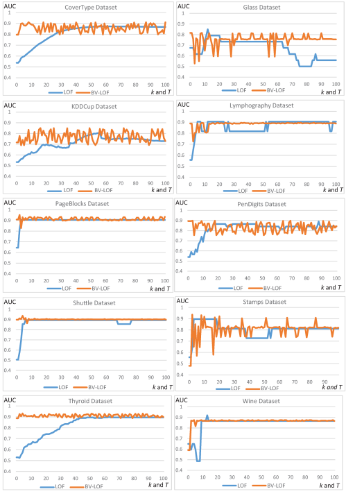
In order to reveal the influences of parameters on the algorithms, BV-LOF and LOF methods are compared in the experiment, where both the parameter k of LOF and the parameter T of BV-LOF change from 1 to 100. The boxplots in Figure 7 show the changes of AUC values with different size of the neighborhood (k) for the LOF algorithm and with different ensemble size (T) for the BV-LOF algorithm on 10 datasets. It can be seen that, for the LOF algorithm, k values smaller than 10 generally tend to result in poor detection of outliers. However, promising results of BV-LOF sometimes appeared even if small ensemble sizes (T < 10).
It is also possible to say from these results shown in Figure 7 that the point in which the AUC measure reaches to maximum varies according to the dataset used. Namely, both LOF and BV-LOF methods are clearly sensitive to the value of the input parameters. This indicates that the parameter k for the LOF algorithm and the parameter T for the BV-LOF algorithm should be optimized to obtain better detection rates. For some datasets such as PageBlock, Shuttle, Wine, Thyroid, and Lymphography, the BV-LOF method has high stability against changing T, but the results slightly fluctuate for other datasets. According to the results shown in Figure 7, BV-LOF is seen to be least affected by the variation of T for the Shuttle data, while it is more heavily affected by the parameter T for the Stamps and Glass datasets.
In the tests with different k, the AUC ratios of the LOF method generally increase when k value increases and becomes close to 0.9; however, it sometimes tends to increase quickly, but sometimes it tends to increase slowly. One reason is that when the dataset size is large (as for CoverType (286,048 instances), KDDCup (60,632 instances), PenDigits (9,868 instances); Thyroid (3,772 instances)), this generally makes the LOF algorithm more sensitive to the values of k. In this case, the higher k values tend to provide higher AUC rates. On the contrary, the AUC ratio reaches the maximum value more quickly (with the smaller k values) on the datasets with small sizes, such as Wine (129 instances), Lympho-graphy (148 instances), Glass (214 instances), and Stamps (340 instances).
Another interesting fact is that for each k and T, the curve never touches one or zero for both LOF and BV-LOF methods. Hence, there is not a single value for k and T such that all the outliers are correctly covered or all the outliers are not covered.
Table 4 shows the k values that provided the LOF algorithm obtaining the best result and T values (ensemble size) that produced the best AUC score for the BV-LOF method. As mentioned earlier, all the k and T values ranged from 1 to 100 were given as input to those algorithms. The results given in Table 4 indicated that the maximum compromise of BV-LOF generally appeared even if small T values such as T=1 for Glass dataset, T=2 for Stamps dataset, T=3 for PenDigits dataset and T=4 for PageBlocks, Shuttle and Thyroid datasets. However, for the LOF algorithm, k values smaller than 10 generally didn’t provide to reach the best AUC value. For instance, the AUC score reached the maximum for the PenDigits dataset when the value of k is 88. The point to which AUC value reaches to maximum varies from dataset to dataset. However, compared to LOF, BV-LOF reaches the maximum AUC ratio with the smaller input parameter, 22.6 versus 37.5 on average.
Figure 7. AUC values obtained from LOF with different k and from BV-LOF with different ensemble sizes (T).
Table 4 The points to which AUC value reaches the maximum for each dataset.
Datasets LOF
Best k Value
BV-LOF
Best T Value
Cover 60 8
Glass 12 1
KDDCup 56 16
Lymphography 54 85
PageBlocks 19 4
PenDigits 88 3
Shuttle 7 4
Stamps 3 2
Thyroid 63 4
Wine 13 99
Average 37.5 22.6
In the BV-LOF approach, the outliers are searched in lower-dimensional subspaces thanks to the feature subset selection, and so this solution attempts to reduce variance by guiding diversity. The integration of partial features is often better than the full features since the combination function at the end recognizes the differential behavior of different subspace samples for a given data point. The multiple feature subspace selection places an important role in improving the performance of an outlier detector and can help to deal with noisy data, to increase robustness and to take the advantages of ensemble learning. Data processing on a lower-dimensional space naturally influences the variance-bias trade-off of the base algorithm (LOF), and so the ensemble framework benefits from the existing variability in each detector. Being based on a two-level ensemble approach to promote diversity, BV-LOF offers an improvement on outlier detection rate, while requiring running time higher than single-level ensemble approaches.

5 Conclusion and future work

In this study, a novel two-level ensemble outlier detection mechanism is proposed. The method consists of two consecutive stages and, at each stage, a different ensemble approach is applied, firstly bagging and then voting. Therefore, it has been called as Bagged and Voted Local Outlier Factor (BV-LOF). In the first stage, the dataset is split into subsets without interfering with instance size in terms of different selection of features. As feature bagging has been proved to produce more robust results by the previous studies, this methodology is used in the first stage. However, it is noticed that the choice of input parameter k (size of the neighborhood) leads to significant differences in LOF performance. Therefore, another ensemble mechanism which is majority voting is applied in the second stage in order to minimize the negative effects of k selection. In that way, the whole system is made more independent from k value selection and combination of distinct kinds of correlated features. The proposed model and base algorithm, Local Outlier Factor (LOF), are applied on 10 benchmark outlier detection datasets with various numbers of iterations and k values to see how much detection capability can be improved with this integration. All the experimental results of BV-LOF were compared with the traditional LOF for each dataset. In the end, it is noticed that this method can be efficiently used for outlier detection. We have also observed that when a few k values generate highly greater separability performance than the rest of the k values, then majority voting becomes unable to reflect the boosted results since there is no weighting mechanism. Finally, the experimental results demonstrate the superiority of the two-level ensemble approach over LOF for the used specific datasets. Since the BV-LOF method includes two-level ensemble operations, it may lead to more computational time than single-level ensemble methods; however, it detects the outliers more robustly. Compared to the traditional LOF outlier detection, the BV-LOF method performs better in identifying outliers and needs no parameter for the neighborhood.
As future work, different kinds of base outlier detectors from different categories (clustering-based, distribution-based, etc.) can be applied in the proposed method. In addition, majority voting could be converted into a weighted form by checking the number of outliers returned from each k value selection in order to take more positive effects of some k values. In this way, AUC scores of the proposed approach can be improved slightly. Furthermore, the BV-LOF approach can be applied to address a specific problem such as fraud detection or erroneous manufacturing parameter detection. Another future work may be conducted by applying the model to datasets that have categorical features. Last of all, the performance of the BV-LOF method can be observed with respect to different outlier densities, so how the results are affected when outliers occupy more space in the whole data can be seen.

Author contributions

Derya Birant (derya@cs.deu.edu.tr) conceived of the presented idea, conducted the literature review and developed the theory. Alican Dogan (alican.dogan@deu.edu.tr) performed the computations and verified the analytical methods. Derya Birant encouraged Alican Dogan to investigate ensemble outlier detection and supervised the findings of this work. Both of the authors discussed the results and contributed to the final manuscript.
1
Aggarwal C.C. (2017). High-Dimensional Outlier Detection: The Subspace Method. In: Outlier Analysis. Springer, Cham.

2
Alshawabkeh M., Jang B., & Kaeli D . ( 2010). Accelerating the local outlier factor algorithm on a GPU for intrusion detection systems. In Proceedings of 3rd Workshop on General Purpose Processing on Graphics Processing Units (pp. 104-110). Pittsburgh, Pennsylvania, USA: ACM.

3
Balamurali M., &Melkumyan A. ( 2018). Detection of outliers in geochemical data using ensembles of subsets of variables. Mathematical Geosciences , 50, 369-380.

4
Bandaragoda T., Ting K., Albrecht D., Liu F., Zhu Y., & Wells J . ( 2017). Isolation-based anomaly detection using nearest-neighbor ensembles. Computational Intelligence, 34, 968-998.

5
Bhatt V., Sharma K.G., & Ram A . ( 2013). An enhanced approach for LOF in data mining. In Proceedings of International Conference on Green High Performance Computing (ICGHPC 2013); Nagercoil, Tamilnadu, India: IEEE. DOI: 10.1109/ICGHPC.2013.6533918

6
Breunig M.M., Kriegel H., Ng R.T., & Sander J . ( 2000). LOF: identifying density-based local outliers. In Proceedings of 2000 ACM-SIGMOD international conference on management of data (pp. 93-104), Dallas, Texas: ACM.

7
Cao D., Deng Z., Zhu M., Yao Z., Dong J., & Zhao R . ( 2017). Ensemble partial least squares regression for descriptor selection, outlier detection, applicability domain assessment, and ensemble modeling in qsar/qspr modeling. Journal of Chemometrics, 31(11), 1-17.

8
Chakraborty D., Narayanan V., & Ghosh A . ( 2019). Integration of deep feature extraction and ensemble learning for outlier detection. Pattern Recognition, 89, 161-171.

9
Chen Z., Yeo C., Lee B., Lau C., & Jin Y . ( 2018). Evolutionary multi-objective optimization based ensemble autoencoders for image outlier detection. Neurocomputing, 309, 192-200.

10
Cheng Z., Zou C., & Dong J . ( 2019). Outlier detection using isolation forest and local outlier factor. In Proceeding of the Conference on Research in Adaptive and Convergent Systems (pp. 161-168), Chongqing, China: ACM.

11
Domingues R., Filippone M., Michiardi P., & Zouaoi J . ( 2018). A comparative evaluation of outlier detection algorithms: experiments and analyses. Pattern Recognition, 74, 406-421.

12
Gan, Z., &Zhou X. ( 2018). Abnormal Network Traffic Detection Based on Improved LOF Algorithm. In Proceedings of 10th International Conference on Intelligent Human-Machine Systems and Cybernetics (pp. 142-145), Hangzhou, China.

13
Goldstein M., &Uchida S. ( 2016). A Comparative Evaluation of Unsupervised Anomaly Detection Algorithms for Multivariate Data. PLoS ONE, 11(4), 1-31.

14
Hu J., Zhu E., Wang S., Liu X., Guo X., & Yin J . ( 2019). An efficient and robust unsupervised anomaly detection method using ensemble random projection in surveillance videos. Sensors, 19, 1-20.

15
Huang H., Qin H., Yoo S., & Yu D . ( 2012). A new anomaly detection algorithm based on quantum mechanics. In Proceedings of ICDM 2012 Brussels, IEEE 12 th International Conference on Data Mining (pp. 900-905), Brussels, Belgium.

16
Kaneko H.( 2018). Automatic outlier sample detection based on regression analysis and repeated ensemble learning,Chemometrics and Intelligent Laboratory Systems, 177, 74-82.

17
Lazarevic A, &Kumar V. ( 2005). Feature bagging for outlier detection. In Proceedings of ACM SIGKDD 2005 Chicago, 11 th International Conference on Knowledge Discovery and Data Mining (pp. 157-166), Chicago, USA.

18
Leng J., &Huang Z. ( 2011). Outliers detection with correlated subspaces for high dimensional datasets, International Journal of Wavelets, Multiresolution and Information Processing, 9(2), 227-236.

19
Li Z., Fang H., & Yan Y . ( 2019). An ensemble hybrid model with outlier detection for prediction of lithium-ion battery remaining useful life.In Proceedings of CCDC 2019 Nanchang, 31 st Chinese Control and Decision Conference, Nanchang, China.

20
Lopes M., Verissimo A., Carrasquinha E., Casimiro S., Beerenwinkel N., & Vinga S . ( 2018). Ensemble outlier detection and gene selection in triple-negative breast cancer data. BMC Bioinformatics, 19, 168-183.

21
Pasillas-Diaz J., &Ratte S. ( 2017). Bagged subspaces for unsupervised outlier detection. Computational Intelligence, 33(3), 507-523.

22
Pokrajac D., Lazarevic A., & Latecki L.J . ( 2007). Incremental local outlier detection for data streams. In Proceedings of the 2007 IEEE Symposium on Computational Intelligence and Data Mining (pp. 504-515), Honolulu, HI, USA: IEEE.

23
Reif M., Goldstein M. ,&Stahl A. &Breuel T.M. (2008). Anomaly detection by combining decision trees and parametric densities. In: Proceedings of 19th International Conference on Pattern Recognition, Tampa, FL, USA, 8-11 Dec. 2008.

24
Qi J., &Chen W. ( 2018). Learning a discriminative dictionary for classification with outliers. Signal Processing, 152, 255-264.

25
Qin J.F., Yang Y., Du H.Y. , &Hong Z.J., (2019). Outlier detection for on-line monitoring data of transformer based on wavelet transform and weighted LOF. In: 4th International Conference on New Energy and Future Energy System (NEFES 2019); Macao; China; 21-24 July 2019, IOP Conference Series: Earth and Environmental Science, 354(1), 1-10.

26
Salehi M., Leckie C., James B., Vaithianathan T., & Zhang X . ( 2016). Fast Memory Efficient Local Outlier Detection in Data Streams. IEEE Transactions on Knowledge and Data Engineering, 28(12), 3246-3260.

27
Su S., Xiao L., Zhang Z., Gu F., Ruan L., Li S., He Z., Huo Z., Yan B., Wang H., & Liu S . ( 2017). N2DLOF: A New Local Density-Based Outlier Detection Approach for Scattered Data. In Proceedings of IEEE 19th International Conference on High Performance Computing and Communications (pp. 458-465), Bangkok, Thailand. N2DLOF: A New Local Density-Based Outlier Detection Approach for Scattered Data.

28
Sun C., Li Q., Cui L., Yan Z., Li H. ,&Wei W.(2015).An Effective Hybrid Fraud Detection Method. In: Zhang S., Wirsing M., Zhang Z. (eds.) Knowledge Science, Engineering and Management.KSEM 2015. Lecture Notes in Computer Science, 9403. Springer, Cham.

29
Tang B., &He H. ( 2017). A local density based approach for outlier detection. Neurocomputing, 241, 171-180.

30
Tang J., &Ngan H.Y.T. ( 2016). Traffic outlier detection by density-based bounded local outlier factors. Information Technology in Industry, 4(1), 6-18.

31
Wang B., &Mao Z. ( 2019). Outlier detection based on a dynamic ensemble model: applied to process monitoring. Information Fusion, 51, 244-258.

32
Wang X.X., &Huang L.W. ( 2007). Research and improvement of GridLOF algorithm in data mining. Modern Computer, 2007-11.

33
Wu H., Tang X., Wang Z., Wu L., Lu M., Wei L., & Zhu J . ( 2018). Probabilistic automatic outlier detection for surface air quality measurements from the china national environmental monitoring network. Advances in Atmospheric Sciences, 35(12), 1522-1532.

34
Yan Y., Cao L., & Rundensteiner E.A . ( 2017). Scalable top-n local outlier detection. In Proceedings of the 23rd ACM SIGKDD International Conference on Knowledge Discovery and Data Mining (pp. 1235-1244), Halifax, NS, Canada: ACM.

35
Yao H., Fu X., Yang Y., & Postolache O . ( 2018). An Incremental Local Outlier Detection Method in the Data Stream. Applied Sciences, 8, 1-19.

36
Zhang J., Li Z., Nai K., Gu Y., & Sallam A . ( 2019). DELR: a double-level ensemble learning method for unsupervised anomaly detection. Konwledge Based Systems, 181, 1-15.

37
Zhou X., Zhao P., Liu Y., & Cui Z . ( 2013). Semi-supervised Based Training Set Construction for Outlier Detection. In Proceedings of International Conference on Cloud Computing and Big Data (pp. 450-454), Fuzhou, China. DOI: 10.1109/CLOUDCOM-ASIA.2013.96

Outlines

/

京ICP备05002861号-43

Copyright © 2023 All rights reserved Journal of Data and Information Science

E-mail: jdis@mail.las.ac.cn Add:No.33, Beisihuan Xilu, Haidian District, Beijing 100190, China

Support by Beijing Magtech Co.ltd E-mail: support@magtech.com.cn