1 Introduction
2 Literature review
3 Methodology
3.1 Searching paths
3.2 Filtering edges
Figure 1. Three possible situations in the application of XIFA algorithm. Note: (a) The source node has only one weighted edge connected to it, and 100% of its strength is allocated on it; (b) Top 20% of weighted edges carry 80% of the strength of source node. (c) Any 50% of weighted edges carry 50% of the strength of source node. |
Table 1 The procedure of network pruning based on XIFA. |
| Procedure | Column Deletion of Input Relations | Row Deletion of Output Relations |
|---|---|---|
| Network |  | |
| Refactoring | 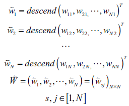 | 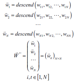 |
| Conditions | 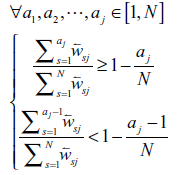 | 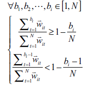 |
| Definition |  |  |
| Pruning |  |  |
| Merging |  | |
| Result |  | |
Note: “descend ()” means to arrange the vectors in descending order. |
3.3 Mixed strategy
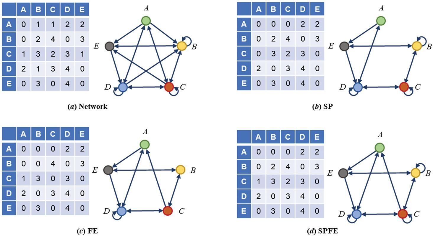
Figure 2. Getting the SPFE from an original network. |
4 Data and modeling
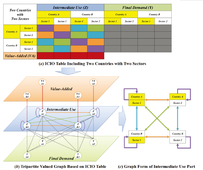
Figure 3. Relations between ICIO table, multi-layer and single-layer ICIO network. |
Table 2 The basic information of ICIO databases. |
| Database | Version | Time Span | Country / Region | Industrial Sector | Abbr |
|---|---|---|---|---|---|
| WIOD | 2016 Release | 2000-2014 | 44 | 56 | WIOD2016 |
| 2013 Release | 1995-2011 | 41 | 35 | WIOD2013 | |
| OECD-TiVA | 2020 Release | 1995-2018 | Unknow | Unknow | TiVA2020 |
| 2018 Release | 2005-2015 | 65 | 36 | TiVA2018 | |
| 2016 Release | 1995-2011 | 64 | 34 | TiVA2016 | |
| 2015 Release | 1995, 2000, 2005, 2008-2011 | 62 | 34 | TiVA2015 | |
| Eora-MRIO | V199.82 | 1990-2015 | 189 | 26 | Eora26 |
| ADB-MRIO | Updated to 2019 | 2000, 2007-2019 | 63 | 35 | ADB2019 |
Note: In addition to sovereign states, the Rest of World (RoW) is taken as an independent economic entity in WIOD, OECD and ADB, most of which belong to the developing countries; In TiVA2018, for “intermediates”, “value added” and “output”, data for Mexico and China are split into MX1, MX2 and CN1, CN2, respectively. |
Table 3 Illustration of properties of the original networks. |
| Networks | |E| | 〈d〉 | 〈K〉 | 〈C〉 |
|---|---|---|---|---|
| GIVCN-WIOD-SC4-2014 | 30,795 (30,976) | 1.006 (1.000) | 174.972 (176.000) | 1.000 (1.000) |
| GIVCN-TiVA-SC4-2014 | 66,600 (67,600) | 1.007 (1.000) | 257.143 (260.000) | 0.996 (1.000) |
| GIVCN-Eora-SC4-2014 | 571,536 (571,536) | 1.000 (1.000) | 756.000 (756.000) | 1.000 (1.000) |
| GIVCN-ADB-SC4-2014 | 57,761 (63,504) | 1.069 (1.000) | 231.972 (252.000) | 0.971 (1.000) |
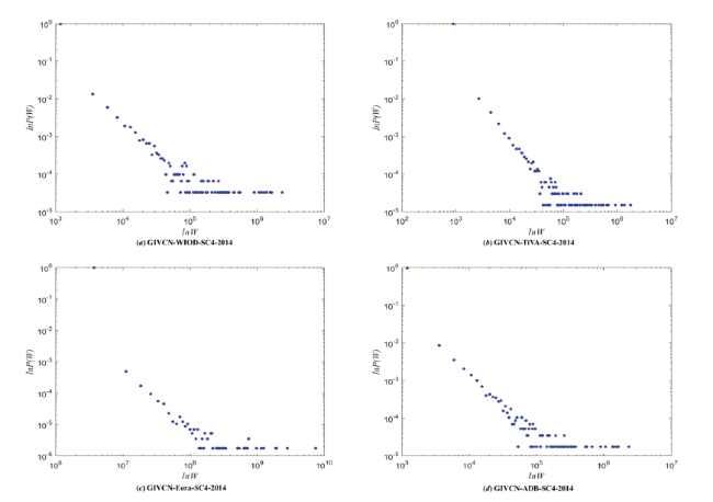
Figure 4. Edge weight distribution of ICIO networks under the double logarithmic coordinate. |
5 Results and discussions
5.1 Preservation of structural information
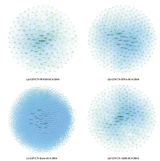
Figure 5. MDS of GIVCN-SPFE-2014 models. Note: EG denoted by the green line is the intersection of ESP and EFE 𝐸𝐹𝐸, i.e., EG = EFE ∩ ESP; EB denoted by the blue line is the edge set only belonging to EFE but not ESP, i.e., EB = EFE - EG; ER denoted by the red line, contrary to EG, is the edge set only belonging to ESP but not EFE, i.e., ER = ESP - EG. |
Table 4 Structural similarity of various backbones and original network. |
| Networks | Nt% no self loops | QAP | ||||||||
|---|---|---|---|---|---|---|---|---|---|---|
| GT | DF | SP | FE | SPFE | GT | DF | SP | FE | SPFE | |
| GIVCN-WIOD-SC4-2014 | 88.068 | 100.000 | 100.000 | 100.000 | 100.000 | 1.000 | 0.998 | 0.994 | 1.000 | 1.000 |
| GIVCN-TiVA-SC4-2014 | 91.539 | 99.615 | 99.615 | 99.615 | 99.615 | 1.000 | 0.991 | 0.996 | 1.000 | 1.000 |
| GIVCN-Eora-SC4-2014 | 65.079 | 100.000 | 100.000 | 100.000 | 100.000 | 1.000 | 1.000 | 0.999 | 1.000 | 1.000 |
| GIVCN-ADB-SC4-2014 | 77.778 | 98.413 | 98.810 | 98.810 | 98.810 | 1.000 | 0.998 | 0.996 | 1.000 | 1.000 |
5.2 Preservation of functional information
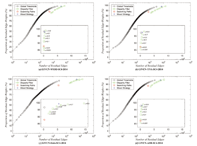
Figure 6. Comparative result of network pruning of GIVCN models. Note: Since the pruning results of SPFE and FE method are almost the same in our models, the FE method is not shown in the figure. |
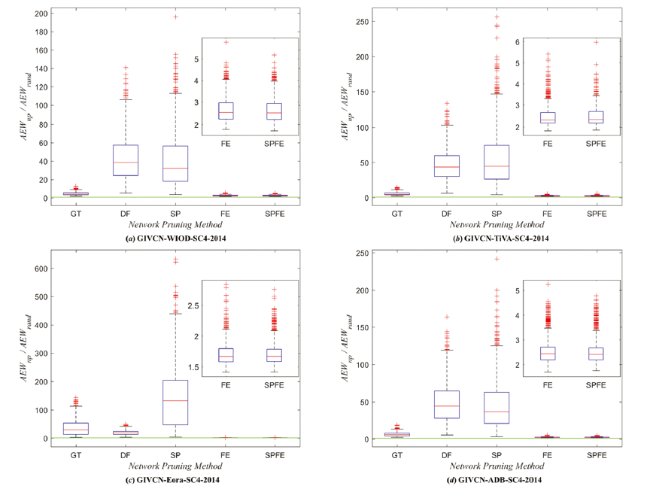
Figure 7. The ratio of the average edge weight of the pruning methods and the null model. |
6 Conclusions
Acknowledgment
Author contributions
Appendix
Table 5 Illustration of properties of the GT backbone. |
| Database | |E| | 〈d〉 | 〈K〉 | 〈C〉 |
|---|---|---|---|---|
| WIOD | 2,009 | 5.4774 | 6.9659 | 0.5291 |
| TiVA | 3,211 | 4.3517 | 8.5598 | 0.4798 |
| Eora | 2,779 | 4.1916 | 43.8587 | 0.4397 |
| ADB | 2,361 | 4.2087 | 8.0484 | 0.4858 |
Table 6 Illustration of properties of the DF backbone. |
| Database | |E| | 〈d〉 | 〈K〉 | 〈C〉 |
|---|---|---|---|---|
| WIOD | 1,385 | 5.4774 | 6.9659 | 0.5291 |
| TiVA | 2,471 | 4.3517 | 8.5598 | 0.4798 |
| Eora | 33,289 | 4.1916 | 43.8587 | 0.4397 |
| ADB | 2,224 | 4.2087 | 8.0484 | 0.4858 |
Table 7 Illustration of properties of the SP backbone. |
| Database | |E| | 〈d〉 | 〈K〉 | 〈C〉 |
|---|---|---|---|---|
| WIOD | 533 | 4.8292 | 2.3864 | 0.4569 |
| TiVA | 806 | 4.9457 | 2.4093 | 0.3788 |
| Eora | 2,496 | 5.1258 | 2.6481 | 0.5381 |
| ADB | 752 | 4.7738 | 2.3695 | 0.4463 |
Table 8 Illustration of properties of the FE backbone. |
| Database | |E| | 〈d〉 | 〈K〉 | 〈C〉 |
|---|---|---|---|---|
| WIOD | 3,825 | 1.9275 | 20.8125 | 0.6231 |
| TiVA | 7,477 | 1.9451 | 27.8764 | 0.6258 |
| Eora | 54,747 | 1.9504 | 71.4762 | 0.5985 |
| ADB | 6,288 | 1.9675 | 24.3253 | 0.616 |
Table 9 Illustration of properties of the SPFE backbone. |
| Database | |E| | 〈d〉 | 〈K〉 | 〈C〉 |
|---|---|---|---|---|
| WIOD | 3,825 | 1.9275 | 20.8125 | 0.6231 |
| TiVA | 7,477 | 1.9451 | 27.8764 | 0.6258 |
| Eora | 54,753 | 1.9485 | 71.4841 | 0.5993 |
| ADB | 6,288 | 1.9675 | 24.3253 | 0.616 |


