1 Introduction
2 Related work
3 Data
Table 1 Selected features from the Altmetrics dataset. |
| Feature | Description |
|---|---|
| Scopus subject | Subject of a research article. |
| Article title | Title of a research article. |
| Article abstract | Abstract of a research article. |
| Abstract length | Number of words in the abstract of a research paper. |
| Follower count | Number of followers a Twitter user has. |
| Author count | Number of authors credited on the research article. |
| Tweet | Tweet about a research article. |
Table 2 Derived features from the dataset. |
| Original feature | Derived feature | Description |
|---|---|---|
| Article title | Title sentiment | Sentiment score of the title of a research article. |
| Article abstract | Abstract sentiment | Sentiment score of a research article abstract. |
| Follower count | Tweet reach | The mean number of followers of each user who tweeted about the research article (i.e. one article can be tweeted by many users, who may differ from each other in the number of followers they have). |
| Tweet | Tweet sentiment | Sentiment score of a tweet related to a research article. |
Figure 1. Number of tweets related to research articles for the years 2011-2017. |
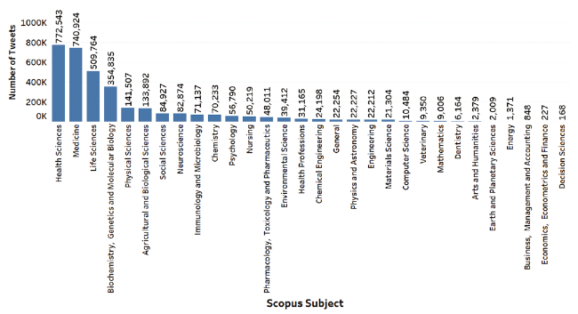
Figure 2. Number of tweets for each Scopus subject. |
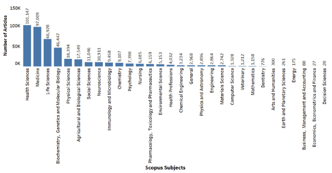
Figure 3. Number of articles for each Scopus subject. |
Table 3 Top 25 positive and negative words in title, abstract, and tweets of research articles. |
| Title | Abstract | Tweets | |||
|---|---|---|---|---|---|
| Positive | Negative | Positive | Negative | Positive | Negative |
| best | boring | awesome | awful | awesome | awful |
| delicious | devastating | best | bleak | best | bleak |
| excellent | disgusting | delicious | boring | breathtaking | boring |
| greatest | evil | excellent | cruel | delicious | cruel |
| perfect | grim | exquisite | devastating | delightful | devastating |
| superb | vicious | flawless | disgusted | excellent | disgusting |
| wonderful | worst | greatest | dreadful | exquisite | dreadful |
| brilliant | fearful | impressed | evil | greatest | evil |
| ideal | repellent | legendary | grim | impressed | grim |
| incredible | retard | magnificent | gruesome | legendary | gruesome |
| beautiful | base | marvelous | horrible | magnificent | horrible |
| splendid | bloody | masterful | horrific | marvelous | horrific |
| attractive | doubtful | perfect | hysterical | masterful | hysterical |
| experienced | filthy | superb | insane | perfect | insane |
| expressive | grief | wonderful | insulting | priceless | insulting |
| favored | hate | artesian | menacing | superb | miserable |
| great | violent | brilliant | outrageous | wonderful | nasty |
| happy | stupid | ideal | ruthless | brilliant | outrageous |
| intelligent | tragic | incredible | shocking | ideal | pathetic |
| joy | sick | beautiful | terrible | incredible | shocking |
| proud | anger | attractive | terrifying | beautiful | terrible |
| uncommon | crude | brave | vicious | splendid | terrifying |
| unforgettable | frustrated | elect | worst | attractive | vicious |
| win | painful | experienced | fearful | brave | worst |
| remarkable | shocked | expressive | hated | elect | fearful |
4 Methods
Table 4 Sentiment distribution of articles using SentiStrength and Sentiment140 libraries. |
| Sentiment library | Metric for multiple sentiments | Number of positive sentiments | Number of negative sentiments | Number of neutral sentiments |
|---|---|---|---|---|
| SentiStrength | mean | 11,443 (≈ 7.7%) | 31,212 (≈ 21%) | 106,057 (≈ 71.3%) |
| SentiStrength | median | 14,905 (≈ 10%) | 39,091 (≈ 26.3%) | 94,716 (≈ 63.7%) |
| Sentiment140 | mean | 3,528 (≈ 2.4%) | 6,254 (≈ 4.2%) | 138,930 (≈ 93.4%) |
| Sentiment140 | median | 3,544 (≈ 2.4%) | 3,168 (≈ 2.1%) | 142,000 (≈ 95.5%) |
5 Results
5.1 Classification models
Table 5 Segregation of sentiments score. |
| Score range | Sentiment |
|---|---|
| [-1,0) | Negative |
| 0 | Neutral |
| (0,1] | Positive |
Table 6 Examples of sentiment label assignment. |
| Article | 1st Tweet and Sentiment | 2nd Tweet and Sentiment | 3rd Tweet and Sentiment | Mean of tweets' sentiment | Final sentiment class label |
|---|---|---|---|---|---|
| Article 1 | Researchers in Norway investigate mortality risk of individuals after the death of a spouse (-0.7184) | Can you die of a broken heart? If your spouse dies, your death risk substantially increases (-0.9186) | A sad study: spouses much more likely to die after being widowed (-0.885) | -0.8407 | Negative |
| Article 2 | Presentation of the ABC Best Paper Award 2013 to Sherrie Elzey. Read the winning paper (0.9022) | ABC Best Paper Award 2013 goes to lead authors Sherrie Elzey and De-Hao Tsai. Read their article for free (0.9001) | NA | 0.90115 | Positive |
| Article 3 | Latest article from our research team has been published about using School Function Assessment! (0) | Article on using School Function Assessment now online (0) | NA | 0 | Neutral |
Table 7 Sentiments on dataset A using different libraries and metrics. |
| Experiment | Sentiment library | Metric for multiple sentiments | Number of positive sentiments | Number of negative sentiments | Number of neutral sentiments |
|---|---|---|---|---|---|
| case 1 | VADER | mean | 55,833 (≈ 37.5%) | 37,957 (≈ 25.5%) | 54,922 (≈ 36.9%) |
| case 2 | VADER | median | 45,606 (≈ 30.6%) | 32,754 (≈ 22%) | 70,352 (≈ 47.3%) |
| case 3 | TextBlob | mean | 67,035 (≈ 45%) | 16,881 (≈ 11.3%) | 64,796 (≈ 43.6%) |
| case 4 | TextBlob | median | 53,466 (≈ 36%) | 13,748 (≈ 9.2%) | 81,498 (≈ 54.8%) |
Table 8 Sentiments on dataset B using different libraries and metrics. |
| Experiment | Sentiment library | Metric for multiple sentiments | Number of positive sentiments | Number of negative sentiments | Number of neutral sentiments |
|---|---|---|---|---|---|
| case 1 | VADER | mean | 44,866 (≈ 42.4%) | 26,664 (≈ 25.1%) | 34,304 (≈ 32.4%) |
| case 2 | VADER | median | 38,038 (≈ 35.9%) | 23,124 (≈ 21.8%) | 44,672 (≈ 42.2%) |
| case 3 | TextBlob | mean | 54,169 (≈ 51.1%) | 11,841 (≈ 11.1%) | 39,824 (≈ 37.6%) |
| case 4 | TextBlob | median | 45,254 (≈ 42.7%) | 9,551 (≈ 9%) | 51,029 (≈ 48.2%) |
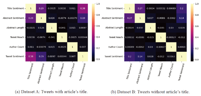
Figure 4. Correlation matrix of features with two class labels - case 4. |
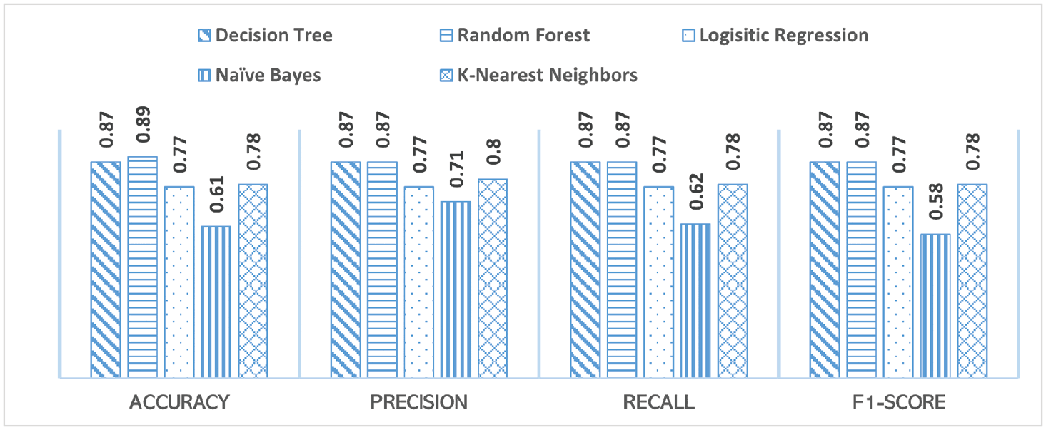
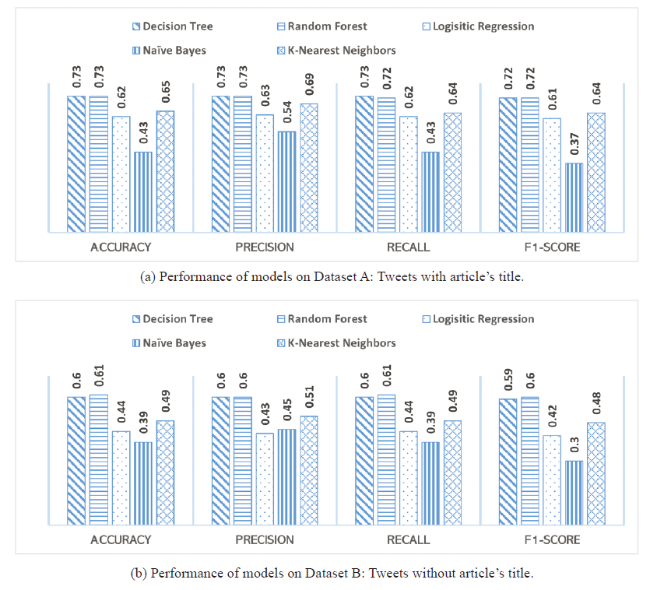
Figure 5. Performance of classification models with two class labels - case 4. |
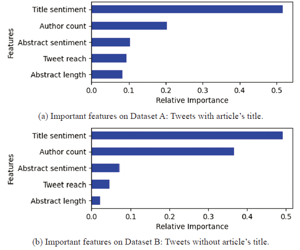
Figure 6. Important features for two-class label classification. |
Table 9 Best results for cases 1-3 with two-class labels. |
| Dataset A: Tweets with article's titles | |||
|---|---|---|---|
| Case Number | Model | Accuracy | F-1 Score |
| 1 | Random Forest | 0.81 | 0.81 |
| 2 | Random Forest | 0.83 | 0.83 |
| 3 | Random Forest | 0.85 | 0.85 |
| Dataset B: Tweets without article's titles | |||
| Case Number | Model | Accuracy | F-1 Score |
| 1 | Random Forest | 0.77 | 0.76 |
| 2 | Random Forest | 0.78 | 0.78 |
| 3 | Random Forest | 0.85 | 0.80 |
Figure 7. Correlation matrix of features with three class labels - case 4. |
Figure 8. Performance of classification models with three class labels - case 4. |
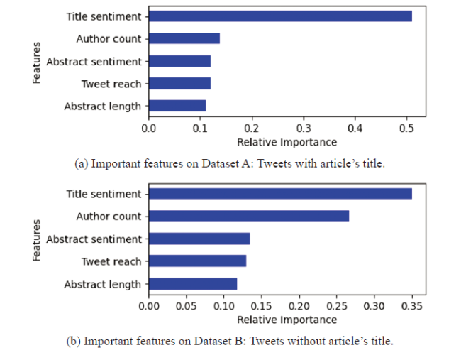
Figure 9. Important features for three-class label classification. |
Table 10. Best results for cases 1-3 with three labels. |
| Dataset A: Tweets with article's titles | |||
|---|---|---|---|
| Case Number | Model | Accuracy | F-1 Score |
| 1 | Random Forest | 0.46 | 0.46 |
| 2 | Random Forest | 0.49 | 0.45 |
| 3 | Random Forest | 0.68 | 0.66 |
| Dataset B: Tweets without article's titles | |||
| Case Number | Model | Accuracy | F-1 Score |
| 1 | Random Forest | 0.46 | 0.45 |
| 2 | Random Forest | 0.47 | 0.44 |
| 3 | Random Forest | 0.56 | 0.56 |
5.2 Regression models
Table 11. Results of the regression models. |
| Dataset A: Tweets with article's titles | ||
|---|---|---|
| Model | Mean Squared Error | R-Squared |
| Multiple Linear Regression | 0.091 | 0.008 |
| Decision Tree | 0.189 | -1.051 |
| Random Forest | 0.104 | -0.130 |
| Support Vector Regression | 0.093 | -0.014 |
| Dataset B: Tweets without article's titles | ||
| Model | Mean Squared Error | R-Squared |
| Multiple Linear Regression | 0.104 | 0.006 |
| Decision Tree | 0.470 | -1.095 |
| Random Forest | 0.119 | -0.133 |
| Support Vector Regression | 0.106 | -0.009 |


