Research Paper

Practical operation and theoretical basis of difference-in-difference regression in science of science: The comparative trial on the scientific performance of Nobel laureates versus their coauthors

  • Yurui Huang ,
  • Chaolin Tian ,
  • Yifang Ma ,
Expand
  • Department of Statistics and Data Science, Southern University of Science and Technology, Shenzhen 518055, Guangdong, China
Yifang Ma (Email: ).

Received date: 2022-12-30

  Accepted date: 2023-01-04

  Online published: 2023-02-22

Abstract

Purpose: In recent decades, with the availability of large-scale scientific corpus datasets, difference-in-difference (DID) is increasingly used in the science of science and bibliometrics studies. DID method outputs the unbiased estimation on condition that several hypotheses hold, especially the common trend assumption. In this paper, we gave a systematic demonstration of DID in the science of science, and the potential ways to improve the accuracy of DID method.

Design/methodology/approach: At first, we reviewed the statistical assumptions, the model specification, and the application procedures of DID method. Second, to improve the necessary assumptions before conducting DID regression and the accuracy of estimation, we introduced some matching techniques serving as the pre-selecting step for DID design by matching control individuals who are equivalent to those treated ones on observational variables before the intervention. Lastly, we performed a case study to estimate the effects of prizewinning on the scientific performance of Nobel laureates, by comparing the yearly citation impact after the prizewinning year between Nobel laureates and their prizewinning-work coauthors.

Findings: We introduced the procedures to conduct a DID estimation and demonstrated the effectiveness to use matching method to improve the results. As a case study, we found that there are no significant increases in citations for Nobel laureates compared to their prizewinning coauthors.

Research limitations: This study ignored the rigorous mathematical deduction parts of DID, while focused on the practical parts.

Practical implications: This work gives experimental practice and potential guidelines to use DID method in science of science and bibliometrics studies.

Originality/value: This study gains insights into the usage of econometric tools in science of science.

Cite this article

Yurui Huang , Chaolin Tian , Yifang Ma . Practical operation and theoretical basis of difference-in-difference regression in science of science: The comparative trial on the scientific performance of Nobel laureates versus their coauthors[J]. Journal of Data and Information Science, 2023 , 8(1) : 29 -46 . DOI: 10.2478/jdis-2023-0003

1 Introduction

In recent decades, with the availability of the growing number of large-scale scientific corpus, researchers in the areas of science of science and bibliometrics are trying to touch the challenging problems in science policy (Bourdieu, 2004; Broadus, 1987; Fortunato et al., 2018; Price, 1986). For example, the development of measures to quantify the impact of science (Uzzi et al., 2013; Wang et al., 2013) and the performance of scientists (Hirsch, 2005; Petersen et al., 2014; Sinatra et al., 2016), the evolution patterns of science and technology system (Huang et al., 2020; Jin et al., 2021; Ma & Uzzi, 2018), the career development of scientists (Ma et al., 2020; Petersen, 2018; Petersen et al., 2014; Yang et al., 2019), etc.
In general, research in science of science is based on empirical data, which lacks natural experiments. To answer some research questions clearly and accurately, econometric models for causality like the difference in difference (DID) are increasingly needed to conduct a quasi-experimental design based on the empirical data. A typical case is the evaluation of the impact of external factors on the future development of scientists. There are already lots of works in science of science that benefit from these econometric models. For example, Azoulay et al. (2010) found that losing scientific superstardom in the collaboration network will decrease the coauthors' future performance, and the attention decay of articles and scientists after the prizewinning of their neighboring articles or scientists. Jin et al. (2021) found that the research topics that have periodic prize conferment are growing quickly and attracting more new scientists.
Unlike natural experiments which can be intended to be random experiments and nearly devoid of confounders' effects, when we process and analyze observational data, we must consider the potential confounding bias. The common method for evaluating the treatment effect is, for instance, to classify individuals from observational data into the treated group and the control group. The treated group consists of individuals exposed to treatment while the control did not. Matching techniques are used to obtain unbiased estimates of treatment effect (Blackwell et al., 2009; Coca-Perraillon, 2007; Hill & Reiter, 2006; Iacus et al., 2012; Rosenbaum & Rubin, 1983; Rubin, 2005). These methods frequently serve as preparation for regression modeling, which is also used in science of science and bibliometrics (W. Li et al., 2019; Liu & Hu, 2022; Ma et al., 2020), was used to choose people from the entire population who will make up the control group. These people will share the same (ideally) features as the treatment group, except for the feature we want to evaluate. For instance, W. Li et al. (2019) found that coauthoring with a prestigious scientist in the earlier career stage will boost a scientist's future scientific performance by comparing the scientists' future performance who collaborate with top scientists with scientists without top-tier coauthors, given other observable features comparable. Usually, two widely used matching methods, propensity score matching (PSM) and coarsened exact matching (CEM), are preferred due to the convenience and the well-established communities and packages.
In this work, we are trying to give a practical recommendation on the DID method and using the common statistical matching approaches to improve the estimation, in science of science. For the practical problem, we will evaluate the status spillovers of prizewinning—how winning a scientific prize affects the winner's future scientific performance compared to her/his collaborators who coauthored the prizewinning paper. The sample experiment we run in this paper is based on the Nobel prize dataset collected by Li et al. (2019), which provides details on the 545 Nobel laureates in the disciplines of physics, chemistry, and medicine who have won the Nobel prizes. At first, we applied DID model to estimate the post-win effects of the Nobel laureates' extra increment of career citations after prizewinning compared to their coauthors. Furthermore, to eliminate the other potential confounders, the control group is further refined through CEM or PSM on the condition that the control scientists (coauthors) did not win but had academic credentials and scientific accomplishments comparable to those of winners. We also gave the conditions, advantages, and possible pitfalls of using DID and matching methods in science of science studies.

2 Difference-in-Difference regression modeling

Natural experiments would limit the impacts caused by various confounders so that it is suitable to study the causes of important events. However, the data available in the real world, for example, the large-scale scientific corpus used in science of science, are observational, and experimenting is time and cost-consuming, which makes it essential to find a solution to the endogenous problem beforehand. The DID approach is thus a widely used methodology to determine the causal relationship in observational studies (Roth et al., 2022).
Let's take a typical example, researchers are given the GDP fluctuation of a country in cities level over years in which there is an earthquake taking place if they want to know how severe an earthquake affects a city's GDP. Cities affected by this catastrophe would have a period of declining GDP following the earthquake. However, because of the global economic and trade scenario, cities in this nation would have had hardships in the years following the earthquake. Therefore, it is difficult to pinpoint the exact causes of the GDP decline.
Assume that cities would or would not experience the earthquake belong to the treatment group and control group respectively. Since it is impossible to predict when and where an earthquake will occur. It is also against ethics, especially in research on diseases, policies, etc. for us to run an experiment that some cities that are randomly assigned to suffer an earthquake while others do not. Once their GDP variation curves coincide or can coincide after translation with each other. DID model evaluate the estimated post-earthquake difference in GDP through fixed effect regression. If this difference is statistically significant, we could declare that earthquake is the direct causal consequence of the occurrence of this event. Based on observational data, the DID approach seeks to address this type of problem practically. In the domains of statistics, economics, and public policy, it is frequently employed. The difference between dependent variables before and after the intervention is of interest to researchers. The time-varying results of the control group served as a baseline for the treatment group, showing the development trend that would occur naturally in the absence of intervention. On the Roy-Rubin Model's foundation, we employ the DID model: Inferring how a treatment affects a person's outcome by looking at how that person could have done in the absence of the treatment (Rubin, 2005).

2.1 Notation

Assume individuals in a set of observational data as I. iI is one of the individuals. Y is the outcome variable in direct relationship to the intervention event. Denote t is the timestamp of the observed period in any kind of unit of time. T is the time dummy variable that equals 0 when t≤0 and 1 when t>0. D is a dummy variable indicating whether individual i is treated, D=1 for individuals of the treatment group, and D=0 for those of the control group. The cross term Tt×Di equals 1 only for the posterior observed outcomes of treated individuals. Covariates Xk (k=1, …, K) are confounders that might influence the dependent variables. They are not asked to be time-varying, for example, in the estimation of earthquake's causal effect on the GDP of cities, covariates could be the locations of cities. Specifically, the potential outcome of an individual i exposed or not to a treatment is given by YiT=DiYiT(1)+(1-Di)YiT(0), where YiT(1) denotes individual i's potential outcome in period T if i is untreated in the first period but exposed to treatment by the second period and YiT (0) denotes individual i's potential outcome in period T if i is untreated in both T=0 and T=1 period.

2.2 Assumptions

Before using the DID regression design, three fundamental premises must be met. The first is the Stable Unit Treatment Value assumption (SUTVA) (Rubin, 1977). SUTVA implies that the outcomes for everyone at any time from observational data are unrelated to any other individuals' treated status. The second is to assume that covariates are not affected by the treatment, i.e., the exogeneity is satisfied. Especially in DID, there is one additional assumption that treatment is only active after the treatment time and has no effect on the pre-treatment population (NEPT).
The most important assumption is the common trend assumption (CTA, also known as the parallel trend assumption).
Common trend assumption (CTA):
E(Yi1(0)-Yi0(0)|Di=1)=E(Yi1(0)-Yi0(0)|Di=0)
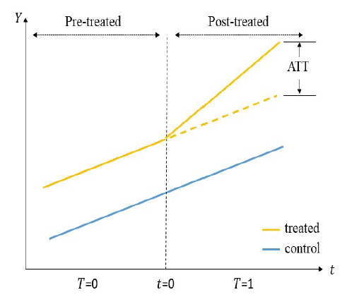
CTA is a core assumption in DID regression design to impute the mean untreated outcomes for the treated group by using the change in outcomes for the untreated group and the baseline outcomes for the treated group. Based on the CTA, it could be stated that the average difference in outcome between the treated and control group remain relatively steady before treatment occurred (Roth et al., 2022). It is so-called parallel rationally therefore that CTA asks for no difference before and after the treated time of untreated units and treated units if they are untreated (See Figure.1). Because the potential outcome of treated individual i when i is untreated is unobservable in practice, the left-hand side of this assumption yields the counterfactual of the trend which does not exist.
Figure 1. Visualized demonstration of the DID regression. Notation is declared in the text.
Another important and often hidden assumption required for the identification of ATT is the no-anticipation assumption, which states that the treatment has no causal effect before its implementation.
No anticipatory effects assumption (NAE):
Yi1(0)=Yi1(1) ∀ i s.t. Di=1.

2.3 Models

2.3.1 Models setting

The difference-in-difference regression model is defined as:
Yit=α+β*Di*Tt+γ1Di+γ2Ttit,
where α is a constant, β is the coefficient of the interaction term, γ1 and γ2 are coefficients of treatment and timing terms respectively. ϵit is the randomized biased term correlated with time t and unit i. According to the assumptions mentioned before and propositions of linear regression, we also give the conditions:
1. E[ϵi]=0
2. The error term ϵi is uncorrelated with the other variables.
From this model, the statistics α, β, γ1 and γ2 could be derived by:
$E[Y_{it}]=E[\alpha]+E[\beta * D_{i} * T_{t}]+E[\gamma_{1}D_{i}]+E[T_{t}]=\alpha + \beta E[D_{i} * T_{t}]+\gamma_{1}E[D_{i}]+\gamma_{2}E[T_{t}].$

2.3.2. Proposition of outcomes

The estimator we are interested in is β, of which the estimated coefficient $\hat{\beta}$ evaluates the difference in average outcome between treatment and control groups before and after treatment time. It is, literally speaking, the difference between treated and untreated groups in the difference between the post-treated period and pre-treated period. The first kind of difference estimator δ1 is based on comparing the average difference in the outcome Yi before and after treatment in the treatment group alone. For simplify, denote E(Y|T=1, D=1) as E(YTD)=E(Y11).
δ1 = E(Y11) - E(Y01)
The second kind of difference δ2 is the average difference in outcome Yi post-treatment between the treatment and control groups, ignoring pre-treatment outcomes.
δ2 = E(Y11) - E(Y10)
The most important kind of difference is the one measuring the gap of the outcome before and after the intervention of treated individuals subtracted by the gap of the outcome before and after the intervention of untreated individuals, i.e., the difference-in-difference estimators:
ATT = ([E(Y11) - E(Y01)] - [E(Y10) - E(Y00)] )=β.
So, the estimated $\hat{\beta}$ of β is the value of the average treatment effect for the treated group (ATET or ATT). The conditional expectations are estimated by observational data from the sample population in practice, such as E(YT=1D=1)= $\bar{Y}_{11}$.

2.4 Limitation of DID

The strong CTA is a well-known limitation of the Difference-in-Differences Method. Figure 1 simply tells the shape of trends when the CTA is satisfied in an observational study. Finding a control group whose trend of outcome is nearly parallel to that of the treatment group before the therapy might be challenging. The optimal scenario is one in which the dependent variable has been well covered by the manually created model and the intervention is the only factor responsible for the difference between the two groups. In practice, the CTA is tested empirically in the procedure of designing a regression model. We can add time and treatment interaction dummy variables before the intervention and evaluate their coefficients. Given that they are not significant and the estimated 95 percent confidence intervals of them cover 0, we could conclude that the difference between comparative groups is insignificant, i.e., trends in the outcome of treatment and control groups are parallel. The CTA, otherwise, is violated if the coefficients of pre-treatment interaction terms are significant, which will result in a biased and invalid estimation.

3 Matching techniques serving for DID

To maintain the reasonability and effectiveness of DID regression model. There are sorts of techniques that could be applied before running DID regression for observational data and study. The matching method is a kind of widely used quasi-experiment, like propensity score and Mahalanobis matching, belonging to a class of matching techniques called Equal Percent Bias Reducing (EPBR). EPBR does not guarantee any level of imbalance reduction in any given dataset, its properties only hold on average across samples, and even then, only by making several typically unprovable assumptions about the method used to generate the data. The imbalance and model dependence may be increased in each application by using these strategies. For our intention, we introduce two popular matching techniques under the framework of the Roy-Rubin Model, coarsened exact matching method (CEM) and propensity score matching (PSM), and how to adopt them as a pre-selection procedure for finding a control group matched for the treatment group in DID regression to as far as possible to minimize selection bias and satisfy the CTA.

3.1 Coarsened exact matching technique

The idea of CEM is first proposed by Iacus et al (2012), which is one of the simplest methods with monotonic imbalance bounding (MIB) properties. The underlying principle of CEM is to coarsen each variable through recoding so that practically indistinguishable values are grouped and given the same numerical value (for example, a continuous variable with numerous distinct values is coarsened into a prespecified number of categories, such as quintiles). Then, according to the coarsened data, the “exact matching” algorithm is used to find matches and prune unmatched groups. The coarsened data are removed, and the original information of the matched data is finally retained.
The CEM algorithm generates a collection of strata, and units in strata that contain at least one treatment, and one control unit are kept in this sample, and units in the remaining strata are removed from this sample. Several criteria and algorithms may be used to create and choose strata. The quantile approach and manual division based on prior experiences are the two most used coarsening techniques. For instance, there are several covariates to consider if we wish to compare a Nobel laureate's scientific innovation to that of a non-prizewinning nominee. These covariates include the research field, career age, publications, and citations, among others. The research field is used as the coarsened variable in this instance; each field group has at least one laureate and several non-prizewinning nominees. The exact matching approach was then used to match the non-prizewinning nominees for laureates. Therefore, even if it is not a perfect match, the treatment field has a match.
Eliminating all imbalances is the task that CEM puts to matching (i.e., differences between the treated and control groups). All multivariate nonlinearities, interactions, moments, quantiles, and other distributional differences above the selected threshold of coarsening are among the imbalances that CEM eliminates. Since the remaining differences all contained small, coarsened strata, a statistical model might be used to bridge them with little risk of model dependence.

3.2 Propensity score matching method

The other famous matching algorithm is PSM, first introduced by Rosenbaum and Rubin (1983). Use the notation yielded in the DID regression model. The performance of PSM has been extensively examined via simulations and theoretical demonstration (Abadie & Imbens, 2006; Austin, 2009). The potential outcome is a variable of interest with covariates X irrespective of the treatment. The conditional independence assumption is to be ensured to eliminate the selection bias. It describes that potential outcomes are independent of treatment assignment when conditioned on the covariates. Another vital assumption is the common support. It rules out the phenomenon of perfect predictability of D given X: 0 < P(D = 1|X) < 1. It ensures that persons with the same X values have a positive probability of being both treated and control individuals (Heckman et al., 1999). Given these two assumptions satisfied, the PSM could be used to estimate the ATT over the common support of treated and control groups (Becker & Ichino, 2002).
Look into the details of PSM, and the canonical steps including choosing an appropriate subset of covariates X. Then the propensity score of everyone is calculated by estimation of the probit or logit regression model. After this step, each individual is assigned a value ready for matching (Coca-Perraillon, 2007). There are several matching algorithms that act as classification estimators including nearest neighbor (NN) (Cover & Hart, 1967), radius matching (Huber et al., 2015), interval matching (Hill & Reiter, 2006), kernel matching and other matching techniques (Garrido et al., 2014). The parameter that received the most attention in evaluation literature is also the average treatment effect on the treated group (ATT) as defined in the former section. In dealing with observational data problems on outcomes independent of time, PSM can estimate the ATT of outcomes and reach conclusions.
For time-dependent outcomes in DID regression models, PSM could only act as a pre-match. In recent years, there has been a trend of natural experiments in the study of economics, management, and medicine. Relevant statistical models have been developed rapidly, among which, PSM-DID is a powerful policy analysis tool. The PSM-DID model is a combination of the propensity score matching model (PSM) and the DID model. Here PSM contributes to the identification of control group individuals as similar as possible to the treatment ones and the DID regression is responsible for the evaluation of the effect caused by treatment. PSM-DID can control individual differences not only generated by observable covariates but also by unobservable covariates when compared with PSM. More than DID, the PSM-DID model takes individual differences into account between the treated group and the control group.
Both CEM and PSM can be taken in priority for more precise and valid estimation results from the DID regression. When the number of observations is too large for PSM to calculate the difference in propensity scores between the treated unit and other control units. In this sense, CEM, as a non-parametric method, performs better than PSM especially when the matching purpose is to find N most similar control units for N treated units, i.e. an N:N match (Wang, 2021). Simple PSM should be avoided unless necessary, such as greedy 1:1 matching without replacement, which matches treated subjects in any order and determines for each one the best match among the unmatched controls. It is advised that researchers carefully plan and design PSM, assess its impact with the knowledge at hand during modeling preparation, and set caliper width considering matching and population biases beforehand (Stuart, 2010).

4 Practical application

4.1 Problem description

In this practice, we are trying to evaluate the status spillovers of prizewinning—how winning a scientific prize affects the winner's future scientific performance compared to her/his collaborators who coauthored the prizewinning paper. For a long time, scientific prizewinning is regarded as a halo for winners, so the winners will benefit a lot in terms of reputation, funding, impact, etc. in the future (Borjas & Doran, 2015; Chan et al., 2014; Merton, 1968). The key to quantitatively evaluating the “halo” effects in future citation impact is to have the proper comparison group. Winners are a special group that has great contributions to science, here we select the winner's collaborators who coauthored the prizewinning works with the winner as the comparison group, so that both the winners and the coauthors have the prizewinning contributions to science, the difference is that one group won the prize and the other group did not. We first used the DID method to estimate the treatment effects, then to further eliminate the other confounding factors like productivity, we applied the CEM and PSM matching before the DID to improve the estimations.

4.2 Data preparation

We used the Nobel prize dataset collected by Li et al. (2019) which provides details on the 545 Nobel laureates in the disciplines of physics, chemistry, and physiology/medicine, including their full list of publications and their representative prizewinning works we then extended the dataset to get all the laureates' coauthors who collaborated the prizewinning works and all scientists' yearly based citations, by using the OpenAlex (https://openalex.org/) corpus.
Our comparison is based on two groups of scientists. According to Nobel prize-winning papers published ranging from 1887 to 2010, the treatment group is made up of Nobel laureates in the field of physics, chemistry, and physiology or medicine with winning years ranging from 1902 to 2016, while their coauthors working in the prizewinning papers are assigned to the control group. We assume that teammates of a prize-winning work share similar capacities and be possessed the same potential to make a breakthrough in their research areas. There are a total of 2,010 scientists in the control group and 635 in the treatment group. To verify our findings, winners who persistently publish papers ten years before and after the year when their studies won the Nobel prize were chosen. Prizewinning works written by a single author are ignored. Eventually, there are 335 laureates and coauthors in total. Table 2 shows the descriptive statistics for our data.
Table 1. Statistics for the treatment effects.
Treatment Control Treatment-Control
Prior E(Y01) E(Y00) E(Y01)-E(Y00)
Posterior E(Y11) E(Y10) E(Y11)-E(Y10)
Posterior-Prior E(Y11)-E(Y01) E(Y10)-E(Y00) [E(Y11)-E(Y01)]-[E(Y10)-E(Y00)]
Table 2. Descriptive statistics for the entire sample (Nobel laureates and their prizewinning-work collaborators).
Prize year Total #Publication Total #Citation
Minimum 1934 10 443
Maximum 2011 1,627 194,896
Mean 1987 245.9 25,662.6
Median 1991 157 13,061
Standard deviation 18.6 266.1 31,571.4
Count 335 335 335

4.3 Modeling

Denote citation impact of a scientist i at a certain year t is Cit. As citations are usually left-skewed distribution (Radicchi et al., 2008), we adopt the rescaled citation impact cit=log(Cit+1). In the first part of modeling, we use the DID regression to calculate the average treatment effect of rescaled citation impact ci for the treated group (ATT), E(ciD=1, T=1)-E(ciD=1, T=0), which is estimated through the regression model:
cit=β0+β1*Treati*Postt+μi+τtit,
Treati is a dummy variable indicating if scientist i is the Nobel laureate or not, it equals 1 when i is the winner and 0 when i is the winner's coauthor. Postt equals 1 when t>0 and 0 otherwise. There are individual fixed effect variable μi and time fixed effect variable τt, so the sole dependent variables Treati and Postt are omitted because they are colinear with fixed effect variables and the coefficients β1 of their cross term Treati*Postt are the ATT we want to estimate. In this problem, we then use the DID regression module in Stata (Donald & Lang, 2007; McCaffrey & Bell, 2003).
According to our selection of the control group, the winner's prizewinning collaborators are supposed to be possessed similar scientific potentials and capacities, then are comparable to the winners before the prizewinning year. So, at first, we could straightforwardly perform a DID regression model on the outcome Y=ci. The result is in table. We can conclude that the difference between the treated group and the control group after the prizewinning years is insignificant, which means that the Nobel prizewinning may not improve the winner's future citations.
However, we found that there is an issue that the common trend assumption of DID is not satisfied. This implies that simply selecting the coauthors of winners is unable to eliminate the effect of the potential endogeneity. One important factor is the different productivities between winners and the coauthor counterparts. In this regard, we used the CEM and PSM to identify coauthors who had been working on their research for a comparable amount of time which is like the winners, i.e., we need to consider their production rate in careers. In detail, t0=0 is the Nobel prizewinning year. Select t1= –10, t2= –5, the matching covariates (number of papers at year t) used in PSM and CEM methods are $p_{it_{1}}$, $p_{it_{2}}$, $p_{it_{0}}$ To maintain the common trend assumption in DID, the average publication in ten years before winning is used, which is numerically defined as $\bar{p_{i}}=\frac{1}{11}\sum_{t=-10}^{0}p_{it}$. The productive capacity of scientists will affect their citation impact to a great extent, so these four covariates are selected for representing the productivity of scientists before the winning year in this experiment. The matching techniques then are applied to find coauthors with similar productivities in the 10-pre-prizewinning years to laureates.
We used Stata to conduct PSM (Leuven & Sianesi, 2003) and CEM (Blackwell et al., 2009) respectively. A k-nearest neighbor algorithm is used in the PSM matching process to offer a matching individual for each treated individual. The coauthors from the PSM-matched control group have the similar productive capability to winners in the ten years prior to prizewinning. Further, we utilize a CEM method on the same set of covariates. Table 3 shows that the pre-treatment citations are becoming closer after we applied the CEM and PSM methods.
Table 3. Matching results by applying different matching techniques.
Average citation index before prizewinning
Matching Techniques - CEM PSM
Group Control Treated Control Treated Control Treated
Observations 227 108 80 80 84 108
Mean 4.7083 5.2350 5.0701 5.2869 5.1353 5.2350
Std. dev. 1.4886 1.5034 1.7627 1.6595 1.5821 1.5034
Minimum 0.3519 0.1997 0 0 1.3754 0.1997
Maximum 8.4902 8.2194 8.3668 8.4933 8.4902 8.2194
As shown in Table 3, using the CEM and PSM substantially eliminated the pre-gaps between treatment groups and control groups. Only 80 pairs of treated and control units with comparable pre-academic productivities remain after CEM, which abandons treated units when matching control units cannot be discovered. For each treatment unit, PSM matches the most comparable control units. The disparities in productivity between the two groups are reduced by these two matching procedures, which also minimizes the promiscuous effects of productivity on citation impacts. Finally, we summarized the results of three DID regression models in Table 4.
Table 4. Regression results and CTA tests by applying different matching techniques.
DID regression Model Results
Model Model I Model II Model III
Matching Techniques - CEM PSM
ATT -0.1488 -0.0780 -0.1481
SE 0.0998 0.1307 0.1317
Common trend assumption Fail Pass Pass
p-value 0.0999 0.6836 0.1582
Fixed Effect Controls
Individual Yes Yes Yes
Year Yes Yes Yes
Given that the CTA is met in Models II and III after combining CEM and PSM with DID, respectively, Table 4 reasonably infers that scientists who have won the Nobel Prize do not witness a noticeable increase in their citation impact as compared to their prizewinning coauthors. When laureates receive Nobel awards, their reputations unquestionably improve in a variety of ways, one of which is an increase in citation impact. However, the prizewinning papers were often works of laureates a long time ago, these milestones' huge potentials had already been recognized and their era significance in pushing the scientific development process had been widely acknowledged. From this perspective, it is not surprising that their citation impacts did not grow after their victory.

5 Discussion

5.1 Summary

In this work, we demonstrated how to use the DID method in science of science studies and how to use the common statistical matching approaches such as PSM and CEM to improve the estimation. We gave detailed definitions of the DID method, and the mathematics behind it we emphasized the conditions before applying the DID method and introduced several matching methods to improve the estimation. As a case study, we studied how winning a scientific prize affects the winner's future scientific performance compared to her/his collaborators who coauthored the prizewinning paper.

5.2 More on DID and when to use matching

The underlying premise of DID is that, in the absence of therapy, the average outcomes for the treated and control groups would have progressed similarly over time. The parallel trends assumption, however, is unrealistic in many health policies, economic, or science of science settings because of potential confounders.
Consider scenarios where the common trend assumption holds, the estimation is unbiased, and the DID estimator provides a clear estimate of the event's expected causal effect. On the other hand, the predicted values should be false positives anytime the CTA is broken because confounding bias exists. In this regard, it is necessary to modify the settings, uncover additional potential factors, and ensure that the CTA is valid before performing the DID regression.
To reduce any potential imbalance between the treatment and control groups, we present two matching strategies in this paper: CEM and PSM. Both alternatives can be used to maintain the CTA. CEM is a nonparametric matching technique that can be used in a quasi-experimental design to compare an outcome over time between two groups. When compared to PSM and used in the context of a comparison group framework, CEM has been demonstrated to produce estimates of the causal effect with lower variance and bias for any sample size (King et al., 2011).
We recommend researchers test both CEM and PSM simultaneously and assess how well they choose the proper control group units for the treatment ones in the CTA test of DID regression. However, PSM is not advised to be used when the size of the control group is significantly bigger than that of the treated group because this will prevent the propensity scores from being calculated due to inadequate processing capability (King & Nielsen, 2019). Especially for 1:1 matches, the CEM performs better than PSM (King et al., 2011). The PSM is advised if we wish to locate control units for each treatment unit without missing any of them because of matching failures. While in CEM, treated units may be abandoned if they were not in some stratum with control units, it would match one or more control units as similarly as feasible to a treated unit.

5.3 Take-home massage

In this section, we summarize the most crucial aspects of using matching techniques in studies that want to apply DID in science of science studies.
$\bullet$ For your study purpose, to estimate the treatment effects of an extreme event, make sure it's proper to use DID method. Create testable hypotheses of interest and determine your dependent, independent, and confounding variables first. List all possible confounders you can find to avoid confounding bias whenever possible.
$\bullet$ Choose the appropriate time variable and decide the time when the intervention happens. Build up balanced or strongly balanced panel outcomes data in a period, which demands that outcome variables of the treated and control groups are observed in each time node during this period.
$\bullet$ Compute and visualize the outcome trends of control and treated groups, if the CTA is satisfied, you could straightforwardly apply a DID regression. Otherwise, you could calculate descriptive statistics for all dependent and independent variables you would use and apply matching techniques or other methods to seek matched control units for treated ones until the CTA is satisfied.
$\bullet$ Estimate the average treatment effect for the treated group and report the estimated coefficients as well as their stand error and confidence intervals and describe the details of your results.

Acknowledgments

We thank OpenAlex for the scientific corpus dataset and Li. et al for the Nobel dataset.

Author contributions

Yurui Huang (12031320@mail.sustech.edu.cn): Methodology, Software, Formal analysis, Writing—original draft, review& editing. Chaolin Tian (12131250@mail.sustech.edu.cn): Methodology, Writing—review & editing. Yifang Ma (mayf@sustech.edu.cn): Conceptualization, Supervision, Project administration, Writing—review &editing.

Conflict of interest statement

The authors have no competing interests.

Funding information

This work was supported by grants from the National Natural Science Foundation of China, with No. NSFC62006109 and NSFC12031005.

Data availability

All data we used in this work is publicly available, with sources linked in the text.
[1]
Abadie A., & Imbens G. W. (2006). Large sample properties of matching estimators for average treatment effects. Econometrica, 74(1), 235-267.

DOI

[2]
Austin P. C. (2009). Some methods of propensity-score matching had superior performance to others: results of an empirical investigation and Monte Carlo simulations. Biometrical Journal: Journal of Mathematical Methods in Biosciences, 51(1), 171-184.

[3]
Azoulay P., Graff Zivin J. S., & Wang J. (2010). Superstar extinction. The Quarterly Journal of Economics, 125(2), 549-589.

DOI

[4]
Becker S. O., & Ichino A. (2002). Estimation of average treatment effects based on propensity scores. The Stata Journal, 2(4), 358-377.

DOI

[5]
Blackwell M., Iacus S., King G., & Porro G. (2009). cem: Coarsened exact matching in Stata. The Stata Journal, 9(4), 524-546.

DOI

[6]
Borjas G. J., & Doran K. B. (2015). Prizes and productivity how winning the fields medal affects scientific output. Journal of human resources, 50(3), 728-758.

[7]
Bourdieu P. (2004). Science of science and reflexivity. Polity.

[8]
Broadus R. N. (1987). Toward a definition of “bibliometrics”. Scientometrics, 12(5), 373-379.

DOI

[9]
Chan H. F., Frey B. S., Gallus J., & Torgler B. (2014). Academic honors and performance. Labour Economics, 31, 188-204.

DOI

[10]
Coca-Perraillon M. (2007). Local and global optimal propensity score matching. SAS Global Forum, https://support.sas.com/resources/papers/proceedings/proceedings/forum2007/185-2007.pdf

[11]
Cover T., & Hart P. (1967). Nearest neighbor pattern classification. IEEE transactions on information theory, 13(1), 21-27.

DOI

[12]
Donald S. G., & Lang K. (2007). Inference with difference-in-differences and other panel data. The review of Economics and Statistics, 89(2), 221-233.

DOI

[13]
Fortunato S., Bergstrom C. T., Börner K., Evans J. A., Helbing D., Milojević S., Petersen A. M., Radicchi F., Sinatra R., & Uzzi B. (2018). Science of science. Science, 359(6379), eaao0185.

DOI

[14]
Garrido M. M., Kelley A. S., Paris J., Roza K., Meier D. E., Morrison R. S., & Aldridge M. D. (2014). Methods for constructing and assessing propensity scores. Health services research, 49(5), 1701-1720.

DOI PMID

[15]
Heckman J. J., LaLonde R. J., & Smith J. A. (1999). The economics and econometrics of active labor market programs. In Handbook of labor economics (Vol. 3, pp. 1865-2097). Elsevier.

[16]
Hill J., & Reiter J. P. (2006). Interval estimation for treatment effects using propensity score matching. Statistics in medicine, 25(13), 2230-2256.

DOI PMID

[17]
Hirsch J. E. (2005). An index to quantify an individual's scientific research output. Proc Natl Acad Sci U S A, 102(46), 16569-16572. https://doi.org/10.1073/pnas.0507655102

DOI

[18]
Huang J. M., Gates A. J., Sinatra R., & Barabási A. L. (2020). Historical comparison of gender inequality in scientific careers across countries and disciplines. Proceedings of the National Academy of Sciences, 117(9), 4609-4616.

DOI

[19]
Huber M., Lechner M., & Steinmayr A. (2015). Radius matching on the propensity score with bias adjustment: tuning parameters and finite sample behaviour. Empirical Economics, 49(1), 1-31.

DOI

[20]
Iacus S. M., King G., & Porro G. (2012). Causal inference without balance checking: Coarsened exact matching. Political analysis, 20(1), 1-24.

[21]
Jin C., Ma Y. F., & Uzzi B. (2021). Scientific prizes and the extraordinary growth of scientific topics. Nature Communications, 12(1), 1-11.

DOI

[22]
King G., & Nielsen R. (2019). Why propensity scores should not be used for matching. Political analysis, 27(4), 435-454.

DOI

[23]
King G., Nielsen R., Coberley C., Pope J. E., & Wells A. (2011). Comparative effectiveness of matching methods for causal inference. Unpublished manuscript, Institute for Quantitative Social Science, Harvard University, Cambridge, MA.

[24]
Leuven E., & Sianesi B. (2003). PSMATCH2: Stata module to perform full Mahalanobis and propensity score matching, common support graphing, and covariate imbalance testing.

[25]
Li J. C., Yin Y. A., Fortunato S., & Wang D. S. (2019). A dataset of publication records for Nobel laureates. Scientific data, 6(1), 1-10.

DOI

[26]
Li W. H., Aste T., Caccioli F., & Livan G. (2019). Early coauthorship with top scientists predicts success in academic careers. Nat Commun, 10(1), 5170. https://doi.org/10.1038/s41467-019-13130-4

DOI PMID

[27]
Liu M. J., & Hu X. (2022). Movers' advantages: The effect of mobility on scientists' productivity and collaboration. Journal of Informetrics, 16(3), 101311.

DOI

[28]
Ma Y. F., Mukherjee S., & Uzzi B. (2020). Mentorship and protege success in STEM fields. Proc Natl Acad Sci U S A, 117(25), 14077-14083. https://doi.org/10.1073/pnas.1915516117

DOI

[29]
Ma Y. F., & Uzzi B. (2018). Scientific prize network predicts who pushes the boundaries of science. Proc Natl Acad Sci U S A, 115(50), 12608-12615. https://doi.org/10.1073/pnas.1800485115

DOI

[30]
McCaffrey D. F., & Bell R. M. (2003). Bias reduction in standard errors for linear regression with multi-stage samples. Quality control and applied statistics, 48(6), 677-682.

[31]
Merton R. K. (1968). The Matthew effect in science: The reward and communication systems of science are considered. Science, 159(3810), 56-63.

PMID

[32]
Petersen A. M. (2018). Multiscale impact of researcher mobility. Journal of The Royal Society Interface, 15(146), 20180580.

DOI

[33]
Petersen A. M., Fortunato S., Pan R. K., Kaski K., Penner O., Rungi A., Riccaboni M., Stanley H. E., & Pammolli F. (2014). Reputation and impact in academic careers. Proc Natl Acad Sci U S A, 111(43), 15316-15321. https://doi.org/10.1073/pnas.1323111111

DOI

[34]
Price D. J. (1986). Little science, big science... and beyond (Vol. 480). Columbia University Press New York.

[35]
Radicchi F., Fortunato S., & Castellano C. (2008). Universality of citation distributions: Toward an objective measure of scientific impact. Proceedings of the National Academy of Sciences, 105(45), 17268-17272.

DOI

[36]
Rosenbaum P. R., & Rubin D. B. (1983). The central role of the propensity score in observational studies for causal effects. Biometrika, 70(1), 41-55.

DOI

[37]
Roth J., Sant'Anna P. H., Bilinski A., & Poe J. (2022). What's Trending in Difference-in-Differences? A Synthesis of the Recent Econometrics Literature. arXiv preprint arXiv:2201.01194.

[38]
Rubin D. B. (1977). Assignment to treatment group on the basis of a covariate. Journal of educational Statistics, 2(1), 1-26.

DOI

[39]
Rubin D. B. (2005). Causal inference using potential outcomes: Design, modeling, decisions. Journal of the American Statistical Association, 100(469), 322-331.

DOI

[40]
Sinatra R., Wang D. S., Deville P., Song C. M., & Barabasi A. L. (2016). Quantifying the evolution of individual scientific impact. Science, 354(6312). https://doi.org/10.1126/science.aaf5239

[41]
Stuart E. A. (2010). Matching methods for causal inference: A review and a look forward. Statistical science: a review journal of the Institute of Mathematical Statistics, 25(1), 1.

[42]
Uzzi B., Mukherjee S., Stringer M., & Jones B. (2013). Atypical combinations and scientific impact. Science, 342(6157), 468-472.

DOI PMID

[43]
Wang D. S., Song C. M., & Barabási A. L. (2013). Quantifying long-term scientific impact. Science, 342(6154), 127-132.

DOI PMID

[44]
Wang J. X. (2021). To use or not to use propensity score matching? Pharmaceutical Statistics, 20(1), 15-24.

DOI

[45]
Yang Y., Chawla N. V., & Uzzi B. (2019). A network's gender composition and communication pattern predict women's leadership success. Proceedings of the National Academy of Sciences, 116(6), 2033-2038.

DOI

Outlines

/

京ICP备05002861号-43

Copyright © 2023 All rights reserved Journal of Data and Information Science

E-mail: jdis@mail.las.ac.cn Add:No.33, Beisihuan Xilu, Haidian District, Beijing 100190, China

Support by Beijing Magtech Co.ltd E-mail: support@magtech.com.cn