1 Introduction
2 Regression discontinuity design
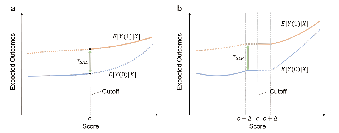
Figure 1. Illustrations of RDD. (a) The continuity framework, and (b) the local randomization framework. The figure depicts the expected outcomes conditional on the running variable Xi, denoted by E[Yi(1)|Xi=x] and E[Yi(0)|Xi=x]. τSRD and τSLR represent the causal effect using these two frameworks at the cutoff c in the window [c−Δ, c+Δ], respectively. This figure is adapted from (Cattaneo & Titiunik, 2022). |
3 The evolution of the regression discontinuity design
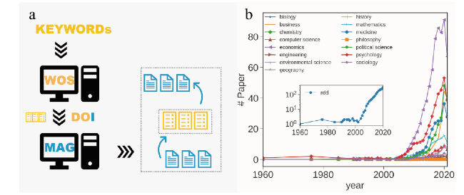
Figure 2. Data collection procedure. (a) Illustration of data collection procedure. Specifically, we manually collect 3,387 RDD papers from Web of Science through keyword searching, and we obtain 2,061 RDD papers in the MAG by matching their DOIs with the Web of Science data. (b) The number of RDD papers in 19 MAG categories as the function of time. The main plot is smoothed using a three-year sliding window. The inset figure shows the total number of RDD papers from 1960 to 2021. |
3.1 The global evolution of RDD papers
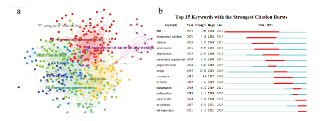
Figure 3. The RDD keyword network and emergent words in WOS. (a) We illustrate the RDD keyword network, where nodes represent keywords and links indicate that two keywords appear in the same paper. The modularity Q is 0.37, indicating a strong community structure. Here, we display only the largest eight clusters, excluding small clusters. (b) Top 15 emergent words of RDD papers, which indicate research frontiers. Year indicates the year when the keyword first appeared, while Begin and End represent the starting and ending years of the keyword as the research frontier. The graph on the rightmost displays the research frontiers in different time periods. For example, air pollution is the research frontier of RDD between 2021 and 2023. |
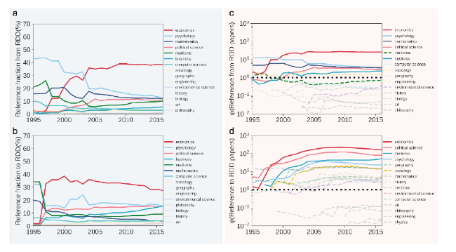
Figure 4. The citation behaviors between RDD and other academic domains over time. (a) The fraction of references made by RDD papers to certain scientific domains. (b) The fraction of references made to RDD papers by papers in various scientific domains. (c) Reference strength from RDD papers to papers in other academic fields. (d) Reference strength from other academic fields to RDD papers. Black dashed lines in c,d represent φ= 1, and other dashed lines in c, d indicate that the strength of references from certain academic fields is lower than the average value cross fields in 2016. |
Table 1. The survey of studies that utilize RDD. Context reveals the settings of the focal paper. Outcome(s) means the dependent variable of the focal paper. Treatment(s) is the treatment variable in the focal paper. In practice, the treatment variable is a binary variable. Running variable(s) is the forcing variable for individuals. |
| Context | Outcome(s) | Treatment(s) | Running Variable(s) | |
|---|---|---|---|---|
| Economics | ||||
| Yi et al. (Yi et al., 2022) | Great Famine in China | Risk tolerance and entrepreneurship in adulthood | Experiencing early-life hardship | Location |
| García-Jimeno et al. (García-Jimeno et al., 2022) | Women’s Temperance Crusade in American | Collective action decisions | Affective information networks | Location |
| Akhtari et al. (Akhtari et al., 2022) | The politically motivated replacement of personnel in the schools in Brazil | The quality of public education provision by the government | Political turnover | Share of Votes |
| Van Der Klaauw (Van Der Klaauw, 2002) | East Coast college’s aid | College enrollment | Offering financial aid | Aid allocation decisions |
| Education | ||||
| Davies et al. (Davies et al., 2018) | Reform of increasing the minimum school leaving age in England | Risk of diabetes and mortality | Remaining in school | Time |
| Huang et al. (Huang & Zhou, 2013) | Great Famine in China | Cognition estimated by episodic memory survey | Completion of primary school | Year of birth and entering primary schooling |
| Clark et al. (Clark & Royer, 2013) | Reform of increasing the minimum school leaving age in England | Adult mortality and health | Remaining in school | Time |
| Science of Science or Innovation Studies | ||||
| Seeber et al. (Seeber et al., 2019) | Scientists’ promotion in Italian higher Education system | Scientists’ number of self-citations | Undergoing the introduction of the habilitation procedure | Time |
| Wang et al. (Y. Wang et al., 2019) | Early-career setback, NIH R01 grant applications | Future Career outcomes | Receiving the R01 grant | Priority score |
| Bol et al. (Bol et al., 2018) | Innovation Research Incentives Scheme for early career scientists, Netherlands | Winning a midcareer grant | Winning the early career award | Evaluation scores |
| Bronzini et al. (Bronzini & Iachini, 2014) | Firms’ R&D subsidy in northern Italy | Investment spending of firms | Receiving funding | Priority score |
| Jacob et al. (Jacob & Lefgren, 2011b) | NIH R01 grant applications | Subsequent publications and citations | Receiving an NIH research grant | Priority score |
| Jacob et al. (Jacob & Lefgren, 2011a) | NIH postdoctoral training grants | Subsequent publications and citations | Receiving an NIH postdoctoral training grant | Priority score |
3.2 The application of RDD to Science of Science
3.3 Areas of research using RDD
4 Practical applications of RDD
4.1 Identification
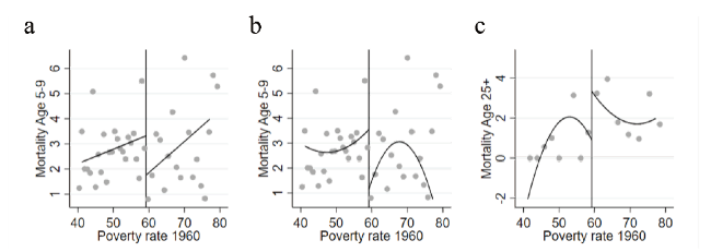
Figure 5. The results of the analysis conducted in (Ludwig & Miller, 2007). (a) - (b) show the linear and quadratic fits, respectively, using rdplot for county mortality of children aged 5 to 9 in 1973-1983. (c) shows the quadratic fit using rdplot for county mortality of people ages 25 and older in 1973-1983. The data used in the analysis come from (Matias D. Cattaneo, 2021). |
4.2 Estimation
4.3 Robustness checks
4.4 A real-world case
Table 2. Counties Characteristic. Column 1 represents county-level data, including the county poverty rate in 1960, mortality of children aged 5 to 9, and people aged 25 and older in 1973-1983. Counties with a 1960 poverty rate of 49.198% to 59.198% are the control group, while counties with a 1960 poverty rate of 59.1984% to 69.1984% are the treatment group, i.e., the poorest counties funded by the HS funding program. |
| County-level data | Counties with 1960 poverty 49.198% to 59.198 | Counties with 1960 poverty 59.1984% to 69.1984 | ||
|---|---|---|---|---|
| No. of observations (counties) | 347 | 228 | ||
| Mean | Std | Mean | Std. | |
| County Poverty Rate 1960 (%) | 54.08 | 2.861 | 63.40 | 2.644 |
| Mortality, Ages 5-9, 1973-1983 (%) | 3.044 | 5.897 | 2.316 | 4.566 |
| Mortality, Ages 25+, 1973-1983 (%) | 132.5 | 30.96 | 135.7 | 30.53 |
Table 3. Regression discontinuity estimation of the effect of HS funding on mortality. Robust standard errors are in parentheses,*** p<0.01, ** p<0.05, * p<0.1. |
| (1) | (2) | (3) | (4) | (5) | ||
|---|---|---|---|---|---|---|
| Parametric | ||||||
| Variable | Mean | Nonparametric estimator | Flexible linear | Flexible quadratic | ||
| Bandwidth or poverty range | 9 | 18 | 36 | 8 | 16 | |
| Main results | ||||||
| Number of countries | 524 | 954 | 2,161 | 482 | 858 | |
| Mortality, Ages 5-9 (%) | 2.252 | -1.895* | -1.198* | -1.114** | -2.201** | -2.558** |
| (0.984) | (0.662) | (0.501) | (1.058) | (1.096) | ||
| Mortality, Ages 25+(%) | 132.626 | 2.204 | 6.016 | 5.872 | 2.091 | 2.574 |
| (5.645) | (4.025) | (3.600) | (5.872) | (6.370) | ||


