Research Papers

Dimensionality reduction model based on integer planning for the analysis of key indicators affecting life expectancy

  • Wei Cui ,
  • Zhiqiang Xu ,
  • Ren Mu ,
Expand
  • School of Statistics, Jilin University of Finance and Economics, Changchun, Jilin 130117, China
†Ren Mu (Email: ).

Received date: 2023-10-19

  Revised date: 2023-11-08

  Accepted date: 2023-11-09

  Online published: 2023-11-29

Abstract

Purpose: Exploring a dimensionality reduction model that can adeptly eliminate outliers and select the appropriate number of clusters is of profound theoretical and practical importance. Additionally, the interpretability of these models presents a persistent challenge.

Design/methodology/approach: This paper proposes two innovative dimensionality reduction models based on integer programming (DRMBIP). These models assess compactness through the correlation of each indicator with its class center, while separation is evaluated by the correlation between different class centers. In contrast to DRMBIP-p, the DRMBIP-v considers the threshold parameter as a variable aiming to optimally balances both compactness and separation.

Findings: This study, getting data from the Global Health Observatory (GHO), investigates 141 indicators that influence life expectancy. The findings reveal that DRMBIP-p effectively reduces the dimensionality of data, ensuring compactness. It also maintains compatibility with other models. Additionally, DRMBIP-v finds the optimal result, showing exceptional separation. Visualization of the results reveals that all classes have a high compactness.

Research limitations: The DRMBIP-p requires the input of the correlation threshold parameter, which plays a pivotal role in the effectiveness of the final dimensionality reduction results. In the DRMBIP-v, modifying the threshold parameter to variable potentially emphasizes either separation or compactness. This necessitates an artificial adjustment to the overflow component within the objective function.

Practical implications: The DRMBIP presented in this paper is adept at uncovering the primary geometric structures within high-dimensional indicators. Validated by life expectancy data, this paper demonstrates potential to assist data miners with the reduction of data dimensions.

Originality/value: To our knowledge, this is the first time that integer programming has been used to build a dimensionality reduction model with indicator filtering. It not only has applications in life expectancy, but also has obvious advantages in data mining work that requires precise class centers.

Cite this article

Wei Cui , Zhiqiang Xu , Ren Mu . Dimensionality reduction model based on integer planning for the analysis of key indicators affecting life expectancy[J]. Journal of Data and Information Science, 2023 , 8(4) : 102 -124 . DOI: 10.2478/jdis-2023-0025

1 Introduction

In the big data era, data related to internet users is characterized by an increasing number of samples and dimensional characteristics. This data plays a pivotal role in diverse fields, including augmented reality, mixed reality, virtual reality, and the anticipated 6G services (Rani et al., 2022). However, as the number of samples and characteristics expands, the complexity of data processing escalates. Hence, utilizing “low-loss” dimensionality reduction (DR) techniques to derive the best low-dimensional data has become a pressing concern in numerous burgeoning domains (Jia et al., 2022). Current DR techniques mainly cater to datasets with many samples. They often directly address the sample’s characteristics, as seen in methods like Principal Component Analysis (PCA), Factor Analysis (FA), and Non-negative Matrix Factorization (NMF) (Roy et al., 2022; Sawant & Bhurchandi, 2022; Yang et al., 2022). These algorithms excel in extracting low-dimensional data from large sample sets. However, in high-dimensional datasets with limited samples, the number of characteristic dimensions exceeding the sample count results in a singular covariance matrix. When applied to high-dimensional data with a smaller sample size, their performance diminishes. Lasso, as a convex optimization method based on the L1 norm, possesses characteristics such as sparse characteristics, data simplification, and reserved subset reduction (Bhadra et al., 2019). It can be applied to extract characteristics from high-dimensional datasets with small samples that exhibit multicollinearity. Though Lasso has found applications in areas such as image recognition and gene analysis (Deutelmoser et al., 2021; Liu et al., 2021), it has no explicit solution. It needs to rely on estimation algorithms for determining regression coefficients diminishes the interpretability of its result.
The Transformer, as a method for extracting characteristic from a global perspective (Vaswani et al., 2017), overcomes the RNN’s limitation of non-parallel computation. Its Attention mechanism also enhances model interpretability. But its proficiency in grasping local details lags behind RNN and CNN. The positional information it uses is an artificial index, lacking flexibility for linear transformations. In summary, current DR techniques often fall short in balancing global information and interpretability, especially in high-dimensional and small-sample datasets. Turning to alternative dimension reduction methods might be the key to rectifying these traditional model limitations.
Clustering stands as a cornerstone tool in data mining applications and research (Ezugwu et al., 2022), occasionally utilized for DR. It’s an unsupervised learning algorithm, that aims to identify natural groupings within a set of patterns, points, or objects (Golalipour et al., 2021). Among the common algorithms, K-Means is computationally efficient but is tailored for convex data (Nasiri et al., 2021). The hierarchical clustering, though more complex, delivers superior accuracy (Tian et al., 2022). In addition, none of these clustering algorithms take the global optimum as the objective function (Golalipour et al., 2021). Each clustering algorithm performs well on suitable data, but for any dataset, selecting the optimal parameters does not always get good performance. For large datasets with outliers, the result obtains by the most complex clustering algorithm do not meet the actual clustering requirements. Therefore, there is an urgent need to develop new characteristic extraction algorithms and validation indicators to produce an accurate and low-complexity model for all realistic data (Oyewole & Thopil, 2023).
In this paper, we construct a new DRMBIP, referring to the four foundational concepts of neighbors, links, objective function, and similarity measure in the ROCK clustering algorithm (Guha et al., 2000). The model takes the correlation of the original data as the similarity measure between the indicators, which solves the problem of solving multidimensional small sample data.
Meanwhile, the model takes maximizing the sum of intra-class correlations, minimizing the sum of inter-class correlations, and minimizing the out-of-bounds penalties as the objective function. It enables the model to find the best neighbors and links in the case of satisfying the inter-class and intra-class correlation threshold.
Specifically, the DRMBIP proposed in this paper has the following four advantages:
◎ More interpretable. In other clustering algorithms such as K-Means, ROCK, DBSCAN, etc., the clustering centers are virtual nodes (Ding & He, 2004; Fahim, 2023; Flegner et al., 2023). However, in the results of the reduced dimensional model in this paper, the class center indicator is real and has accurate practical significance.
◎ No need to consider the number of clusters. The number of clusters can have a huge impact on the effectiveness (Song et al., 2022). The DRMBIP solves this problem, and not only obtains the optimal number of clusters, but also makes the model effect globally optimal.
◎ Automatic elimination of abnormal indicators. In real data, there are indicators that are difficult to classify. And it is unreasonable to force them into a certain class when using clustering algorithms for dimensionality reduction (Wang et al., 2021). In the DRMBIP of this paper, it is possible to perform dimensionality reduction while eliminating a certain number of indicators, which improves the effect of dimensionality reduction.
◎ Easier to view results. The results of the model often face difficulties in visualization. In this paper, the correlation between the indicators is used as the basic data of the model, which can be simpler and more intuitive to display the results of dimensionality reduction in a two-dimensional plane.

2 Literature review

Since this paper focuses on linear and global, common existing dimensionality reduction algorithms can be classified into four categories (Espadoto et al., 2019): Linear & Global, Linear & Local, Nonlinear & Global, and Nonlinear & Local.
Linear & Global uses a linear function that preserves the structure of the pairwise distances between all data samples. Representative algorithms are PCA (Abdi & Williams, 2010), FA (Stephenson, 1935), and NMF (Lee & Seung, 1999). PCA is a dimensionality reduction method that transforms the data variables into a set of linearly uncorrelated variables by applying a linear transformation to the data variables. Scholars have proved that PCA is a continuous solution for the clustering membership indicators in K-Means. It suggests PCA potentially performs clustering (Ding & He, 2004). The difference between FA and PCA is that the former uses variance maximization for dimensionality reduction, while the latter performs DR based on the dependencies between variables. However, NMF decomposes the original data matrix into the multiplication of the base matrix W and the coefficient matrix H, i.e., W×H≈V, it uses the coefficient matrix H instead of the original matrix V to achieve dimensionality reduction.
Linear & Local is to use linear function in the process of dimensionality reduction to preserve local features. The representative algorithms are LLE (Roweis & Saul, 2000), LE (Belkin & Niyogi, 2001), and t-SNE (Van der Maaten & Hinton, 2008). The LLE algorithm involves only matrix operations and is easy to implement, but it is not suitable for closed streaming data. The LE algorithm is less computationally and faster in execution compared to the LLE algorithm, but it is less robust to noise and cannot learn the intrinsic geometric structure from noisy data. The t-SNE algorithm improves the computational efficiency compared to the SNE algorithm, but it has no unique optimal solution and cannot be used for prediction. Currently, the corresponding mainstream linear variants of these three common DR algorithms are LPP (Yao et al., 2023), NPE (Zhang et al., 2023), and t-SNLE (Xia et al., 2021). They alleviate the curse of dimensionality and retain the advantages of cluster separation, but it is difficult to maintain the topological connectivity of the data after dimensionality reduction (Yao et al., 2023).
Nonlinear & Global is the use of nonlinear functions to preserve the structure of the pairwise distances between all data samples. Representative algorithms are nonlinear MDS (Kruskal & Wish, 1978) and ISOMAP (Tenenbaum et al., 2000). The MDS algorithm uses Euclidean distances to measure the distances between samples. It is difficult for the algorithm to represent the true geometric structure in low-dimensional space. The effect of the MDS algorithm using nonlinear function optimization is greatly affected by the chosen function. However, it is difficult to fundamentally improve the shortcomings of the MDS algorithm on nonlinear streaming data. The essence of ISOMAP is consistent with MDS. The difference is that ISOMAP uses Geodesic distances instead of Euclidean distances. The Geodesic distance can more realistically reflect the real low-dimensional geometric structure of the flow shape and better measure the distance between samples.
Nonlinear & Local is the use of nonlinear functions to preserve local features during data dimensionality reduction. Representative algorithms are LLE (Roweis & Saul, 2000), LE (Belkin & Niyogi, 2001), t-SNE (Van der Maaten & Hinton, 2008), and UMAP (McInnes et al., 2018). The UMAP algorithm assumes that the sample data is uniformly distributed in the topological space and can be mapped from these finite data samples to a lower dimensional space. Currently, these techniques are more popular for dimensionality reduction and visual exploration of multidimensional datasets (Xia et al., 2021). For example, t-SNE and UMAP are excellent at separation, but slightly inferior at compactness.
Clustering, as an indispensable tool in data mining, can be used in combination with dimensionality reduction such as PCA (Shuai, 2022; Yang et al., 2022; Yunita et al., 2022), t-SNE (Ullah et al., 2022), and UMAP (Can-can et al., 2022). And it can use alone to reduce the dimensionality of the indicator. The most common practice is to use dimensionality reduction methods to compress the data dimensions locally or globally. And the indicators with lower dimensions can be used in data mining work. It is less common to use clustering alone to reduce indicators. It retains indicators that are highly interpretable and interchangeable, providing high flexibility in dimensionality reduction. However, most clustering algorithms have strict requirements, requiring data to satisfy convexity assumptions and are difficult to handle outliers.
Integer programming, as a very powerful tool for solving the problem of reality today, has a wide range of applications (Achterberg et al., 2020). Advances in research related to data sparsity and matrix decomposition have led to a rapid increase in the solution size of commercial solvers such as Gurobi, Cplex, and Mosek (Li et al., 2020). Moreover, the optimal solution can be solved in reasonable time for large-scale cases. Such as urban traffic light scheduling for pedestrian-vehicle mixed-flow networks (Gupta et al., 2022) and efficient operation of distributed generation networks (Cortés et al., 2018). The wide range of applications and the increasing solution scale of integer linear programming provide opportunities for more and more ideas. Many of the concepts in the ROCK clustering algorithm (Guha et al., 2000) can be expressed using integer programming tools, making it possible to construct a dimensionality reduction model.
In this paper, the data of relevant indicators affecting life expectancy is obtained from the Global Health Observatory (GHO). The data are used as the basis for dimensionality reduction analysis. First, we use the DRMBIP to eliminate the abnormal indicators and obtain the filtered indicators. second, we use the correlation data between the indicators to display results. It visualizes the complex relationship between different types of indicators in two-dimensional plane. Finally, we can combine the correlation results of the model with the original categorization between the indicators for further dimensionality reduction. This allows us to find potentially important factors that influence life expectancy.

3 Dimensionality reduction model based on integer programming

In this section, we will give a description of the parameters and variables. Then, we will focus on the two main models and their mathematical formulas in this paper. Finally, we establish relevant intra-class and inter-class evaluation indexes and introduce some evaluation indexes of traditional clustering models to evaluate the model results comprehensively.

3.1 Description of symbols

To build model of DRMBIP, the following symbol must be introduced:
i denotes the subscript of the indicator
j denotes the subscript of alternative class center
I denotes the set of all subscripts of indicators
J denotes the set of all subscripts of alternative class centers
pnum denotes the number of enabled indicators
pcenter denotes the number of classes in the result
λ denotes the lower limit parameter of intra-class correlation
η denotes the upper limit parameter of inter-class correlation
α1 denotes the weight of the inter-class correlations in the objective function
α2 denotes the weight of intra-class correlations in the objective function
α3 denotes the weight of the part above λ or below η in the objective function
α4 denotes the weight of the difference of ζ and ξ in the objective function
cij denotes the absolute value of the Pearson correlation coefficient between the i-th and j-th indicator
cij' is similar with cij, but cij' takes the value 0 on the diagonal
Define the decision variables as follows:
$x_i=\left\{\begin{array}{l}1 \ \ if\ the \ i-th \ indicator \ is \ selected \ as \ a \ class \ center \\0 \ \ otherwise \end{array}\right.$
$y_{i j}= \begin{cases}1 & if \ the \ i-th \ indicator \ and \ the\ j-th \ class \ center \ are \ same \ class \\ 0 & otherwise \end{cases}$
$z_{i j}=\left\{\begin{array}{l} 1 \ if \ the \ i-th \ and \ the \ j-th \ indicator \ are \ both \ class \ centers \\ 0 \ otherwise \end{array}\right.$
$w_i=\left\{\begin{array}{l} 1 \ if \ the \ i-th \ indicator \ is \ enabled \\ 0 \ otherwise \end{array}\right.$
$e_{i j}^{+}$ denotes the part of the correlation between the i-th and j-th class center that is lower than the parameter λ
$e_{i j}^{-}$ denotes the part of the correlation between the i-th and j-th class center that is higher than the parameter η
ξ denotes the lower limit of intra-class correlation
ζ denotes the upper limit of inter-class correlation

3.2 Dimensionality reduction model based on integer programming

To solve the problem that the number of clusters is difficult to determine, we propose two DRMBIP with reference to the concepts of ROCK clustering algorithm. The DRMBIP uses the correlation as the basic data, the minimum value of the correlation between the indicator and class center is used to measure the compactness. And the correlation between the indicators of class center is used to measure the separation between the classes. In general, multidimensional data in different situations often have different dimensionality reduction requirements. To meet this demand, we set the threshold for measuring the dimensionality reduction as a parameter in DRMBIP-p to improve flexibility.
Objective function (1): minimize the sum of inter-class correlations, maximize the sum of intra-class correlations, and minimize the sum of out-of-bounds penalties, given the weights α1, α2, and α3. Constraint (2): pnum indicators are enabled; Constraint (3): the j-th indicator may be selected as the class center if it is enabled; Constraint (4): the selection of the j-th indicator as the center of the class may result in the attribution of the i-th indicator to same class; Constraint (5): the value of zij is taken to be 1 when the i-th and j-th indicators are used as the center of the class at the same time. In the case of selecting the i-th or j-th indicator alone, the objective function will cause zij to take the value 0; Constraint (6): when classifying the i-th indicator as the j-th class, it is guaranteed that the correlation between the i-th indicator and the class center of the j-th class is as much as possible greater than or equal to λ; and Constraint (7): the inter-class correlation between the class center of the i-th and j-th class is as much as possible less than equal η.
DRMBIP-p:
$\begin{aligned} Minimize \ \ \alpha_1 \sum_{i \in I} \sum_{j \in J} c_{i j}^{\prime} z_{i j}-\alpha_2 \sum_{i \in I} \sum_{j \in J} c_{i j} y_{i j}+\alpha_3 \sum_{i \in I} \sum_{j \in J}\left(e_{i j}^{-}+e_{i j}^{+}\right) \end{aligned}$
$\begin{aligned} {s.t. } & \sum_{i \in I} w_i=p_{ {num }} \end{aligned}$
$\begin{aligned} \sum_{j \in J} y_{i j}=w_i \ \ \ for \ \ all \ \ \ i \in I \end{aligned}$
$\begin{aligned} y_{i j} \leq x_j \ for \ \ all \ \ i \in I, j \in J \end{aligned}$
$\begin{aligned}z_{i j} \geq x_i+x_j-1 \ for \ all \ i \in I, j \in J \end{aligned}$
$\begin{aligned} c_{i j} y_{i j}+e_{i j}^{+} \geq \lambda y_{i j} \ for \ all \ i \in I, j \in J\end{aligned}$
$\begin{aligned} c_{i j}^{\prime} z_{i j}-e_{i j}^{-} \leq \eta z_{i j} \ for \ \ all \ \ i \in I, j \in J \end{aligned}$
$\begin{aligned}& e_{i j}^{-}, e_{i j}^{+} \geq 0 \ for \ \ all \ \ i \in I, j \in J \\ & x_i, w_i, y_{i j}, z_{i j} \in\{0,1\} \ for \ \ all \ \ i \in I, j \in J \end{aligned}$
In DRMBIP-p, the optimal number of clusters can be determined by inputting three parameters: λ, η, and pnum. The introduction of the pnum parameter provides more flexibility for tasks with different requirements. The other two parameters set the dimensionality reduction preference. When preferring compactness, the lower limit of the intra-class correlation λ can be increased and the upper limit of the inter-class correlation η can be appropriately relaxed. Conversely, the upper limit of inter-class correlation η can be reduced, and the lower limit of intra-class correlation λ can be appropriately relaxed to increase inter-class separation when separation is preferred.
In some practical cases, compactness and separation need to be achieved simultaneously. For this purpose, the parameters in Constraint (6) and Constraint (7) in DRMBIP-p can be transformed into variables then the constraints can be linearized. To facilitate comparisons with other models, constraint must be added to control the number of classes in DRMBIP-v.
DRMBIP-v:
$\begin{aligned} Minimize \ \ \ \alpha_1 \sum_{i \in I} \sum_{j \in J} c_{i j}^{\prime} z_{i j}-\alpha_2 \sum_{i \in I} \sum_{j \in J} c_{i j} y_{i j}+\alpha_4(\zeta-\xi) \end{aligned}$
$\text { s.t. } \text { Constraints (2) (3) (4) (5) }$
$\begin{aligned} \sum_{j \in J} x_j=p_{ {center }} \end{aligned}$
$\begin{aligned} c_{i j} y_{i j} \geq \xi-\left(1-y_{i j}\right) \ \ for \ \ all \ \ i \in I, j \in J \end{aligned}$
$\begin{aligned} c_{i j}^{\prime} z_{i j} \leq \zeta+\left(1-z_{i j}\right) \ for \ \ all \ \ i \in I, j \in J \end{aligned}$
$\begin{aligned}& 0 \leq \zeta \leq \xi \leq 1 \\ & x_i, w_i, y_{i j}, z_{i j} \in\{0,1\} \ for \ \ all \ \ i \in I, j \in J\end{aligned}$
Objective function (8): minimize the sum of inter-class correlation, maximize intra-class correlation, and minimize the difference between ζ and ξ. Constraint (9): final clustering into pcenter classes; Constraint (10): when classifying the i-th indicators into the j-th class, ensure that the correlation of the i-th indicators with the class-centered indicators is greater than or equal to ξ; Constraint (11): the inter-class correlation between the i-th and j-th class center is less than or equal to ζ.
The DRMBIP-v differs from DRMBIP-p in that it considers compactness and separation as equally important. Moreover, adding it to the Objective function (8) maximizes ξ and minimizes ζ, resulting in the best dimensionality reduction.

3.3 Evaluation indexes

With reference to the traditional clustering model evaluation indexes, this paper introduces five evaluation indexes, namely, Compactness, Separation, Dunn Validity Index (DVI), Silhouette Coefficient (SI), Davie-Bouldin Index (DBI). In addition, combined with the DRMBIP, seven correlation evaluation indexes for measuring intra-class or inter-class have been established based on the correlation data, which are: minimum intra-class correlation, minimum intra-class and class center correlation, average intra-class correlation, average intra-class and class center correlation, average intra-class correlation (no single class), maximum inter-class correlation, and average inter-class correlation.

3.3.1 Evaluation indexes for traditional clustering models

The formula for calculating the Compactness is as follows:
$Compactness=\frac{\sum_{i \in K} \sum_{j \in C_i} d\left(j, C_i^0\right)}{n}$
which, n denotes the total number of indicators; K={1, …, k}, k denotes the number of classes in the result; d(x, y) denotes the Euclidean distance between indicator x and indicator y; Ci denotes the i-th class; And Ci0 denotes the class center indicator of the i-th class. The Compactness is the average distance from each indicator to the class center indicator. The larger Compactness, the more relevant the indicators within the class and the higher the similarity within the class.
The formula for calculating the Separation is as follows:
$Separation=\frac{\sum_{i, j \in K, i<j} d\left(C_i^0, C_j^0\right)}{C_k^2}$
which, Ck2 is to calculate the number of combinations. The Separation is to calculate the average distance between the centers of each class. A larger Separation denotes that the further apart the classes are, the better the classification is, i.e., the lower the similarity between classes.
The formula for calculating the Dunn Validity Index is as follows:
$\begin{aligned}D V I=\min _{i=1, \ldots, k}\left\{\min _{j=i+1, \ldots, k}\left[\frac{d_1\left(C_i, C_j\right)}{\max _{h=1, \ldots, k} d_2\left(C_h\right)}\right]\right\}\end{aligned}$
which,
$\begin{aligned}d_1\left(C_i, C_j\right)=\min _{x \in C_i, y \in C_j} d(x, y), d_2\left(C_h\right)=\max _{x, y \in C_h} d(x, y)\end{aligned}$
d1(Ci, Cj) denotes the shortest distance between the i-th and j-th class; d2(Ch) denotes the diameter of the h-th class. The DVI is the ratio of the shortest distance between indicators in any two classes to the maximum distance between indicators in any class. Higher DVI values indicate better results.
The formula for calculating the Silhouette Coefficient is as follows:
$\begin{aligned}S I=\frac{1}{k} \sum_{h=1}^k S I_h\end{aligned}$
which,
$\begin{aligned}& S I_h=\frac{1}{\left|C_h\right|} \sum_{i=1}^{\left|C_h\right|}\left[\frac{b_i^h-a_i^h}{\max \left\{a_i^h, b_i^h\right\}}\right], a_i^h=\frac{1}{\left|C_h\right|-1} \sum_{l=1, l \neq i}^{\left|C_h\right|} d\left(x_i^h, x_l^h\right), \\& b_i^h=\min _{j \in\{1, \ldots, k\}, j \neq h}\left\{\frac{1}{\left|C_j\right|} \sum_{l=1}^{\left|C_j\right|} d\left(x_i^h, x_l^j\right)\right\}\end{aligned}$
xih and xlh denote the i-th and l-th indicators of h-th class, respectively; d(xih, xlh) denotes the computation of the Euclidean distance between xih and xlh; aih represents the average distance from the i-th indicator to the other indicators in h-th class; and bih represents the average distance from the i-th indicator in h-th class to the other classes. Corresponding to a sample, SI is the average of all sample SIh. The range of this index is [-1,1], and the closer the samples of the same class to different samples, the higher the score.
The formula for calculating the Davie-Bouldin Index is as follows:
$\begin{gathered}DBI=\frac{1}{k} \sum_{h=1}^k F_{C_h} \end{gathered}$
which,
$\begin{gathered}F_{C_h}=\max _{C_j \neq C_h} F_{C_h C_j}, F_{C_h C_j}=\frac{f_1\left(C_h\right)+f_1\left(C_j\right)}{f_2\left(C_h, C_j\right)}\end{gathered}$
Ch and Cj denote h-th class and j-th class, respectively, and h, j∈{1, …, k}; f1(Ch) denotes the average distance of each indicator in h-th class from the center of the class; And f2(Ch, Cj) denotes the distance between the class centers of h-th class and j-th class. The DBI is used to measure the ratio of the sum of intra-class distances to inter-class distances for any two classes. The smaller DBI, the smaller the intra-class distance, the higher the intra-class similarity, the larger the inter-class distance and the lower the inter-class similarity.

3.3.2 Evaluation indexes for DRMBIP

The dimensionality reduction models proposed in this paper use the correlation as the similarity measure between the indicators. Thus, we can construct evaluation indexes based on the correlation in both intra-class and inter-class aspects. Intra-class compactness based on correlation can be measured in two ways. One way is to calculate the correlation of all two indicators in the class, and the other way is to calculate the correlation between the center of the class and the rest of the indicators.
Minimum intra-class correlation is an indicator used to measure compactness within a class. This indicator is chosen after calculating the minimum correlation between two indicators in each class and then selecting the smallest of them.
The formula for calculating the minimum intra-class correlation is as follows:
${Index}_1=\min _{i \in K}\left\{\min _{x, y \in C_i}[{corr}(x, y)]\right\}$
which, K={1, …, k}, k denotes the number of classes obtained by clustering; corr(x, y) denotes the correlation between indicator x and indicator y.
When adding the constraint of correlation, DRMBIP uses the correlation between the class center and the other indicators. Thus, the intra-class and class center minimum correlation must be calculated to get the actual value under this constraint. The calculation is the same as the calculation of the minimum intra-class correlation, except that when the minimum correlation is calculated, one of the indicators is changed to the class center.
The formula for calculating the minimum intra-class and class center correlation is as follows:
${Index}_2=\min _{i \in K}\left\{\min _{x \in C_i}\left[{corr}\left(x, C_i^0\right)\right]\right\}$
which, $C_i^0$ denotes the class center of i-th class.
Since Index1 and Index2 are susceptible to extreme values, the last step of both can be modified by changing the selection of the minimum value to the average value to eliminate the influence.
The formulas for the average intra-class correlation and the average intra-class and class center correlation are as follows:
$\begin{aligned} { Index }_3 & =\frac{\sum_{i \in K}\left\{\min _{x, y \in C_i}[{corr}(x, y)]\right\}}{k}\end{aligned}$
$\begin{aligned}{ Index }_4 & =\frac{\sum_{i \in K}\left\{\min _{x \in C_i}\left[{corr}\left(x, C_i^0\right)\right]\right\}}{k}\end{aligned}$
If fewer or no indicators are filtered, the quality of indicators may result in a single indicator as one class. The effect of extreme values generated in this case needs to be excluded. Therefore, the calculation of Index3 must be filtered out from the class without a single indicator as one class.
The formula for the average intra-class correlation (not a single class) is as follows:
${ Index }_5=\frac{\sum_{i \in K^{\prime}}\left\{\min _{x, y \in C_i}[{corr}(x, y)]\right\}}{k^{\prime}}$
which, k' denotes the number of elements contained in the set K'; K' denotes the exclusion from K of individual indicators as one class.
While considering the intra-class compactness, the inter-class separation of the results also needs to be considered. For this reason, the maximum inter-class correlation is introduced as a measure of the inter-class separation. The maximum inter-class correlation is susceptible to extreme values, which can be excluded by introducing the average inter-class correlation.
The formulas for the maximum inter-class correlation and the average inter-class correlation are as follows:
${Index}_6=\max _{i, j \in K, i \neq j}\left[{corr}\left(C_i^0, C_j^0\right)\right]$
${ Index }_7=\frac{\sum_{i, j \in K, i<j} {corr}\left(C_i^0, C_j^0\right)}{C_k^2}$
which, $C_k^2$ is to compute the number of combinations.

4 Data and experimental results

Life expectancy is one of the three major human development indexes and a key indicator of the progress of human societies (Baumann, 2021; Sen, 1998). Possession of specific disease-causing genes is not the only reason for contracting diseases (Farhud, 2022). The increase in the vintage of the prescription drugs years has increased the average age of death by 1.23 years in 26 countries (Lichtenberg, 2022), assuming the disease is fixed. Thus, the adequate and advanced medical care is an important means of increasing human life expectancy. However, the uneven distribution of healthcare resources in developed countries due to irrational policies has exacerbated the widening of healthcare inequalities (Alexiou et al., 2021). In the specific period of the COVID-19 pandemic, this inequality was even more obvious, which seriously affected the population’s health and economic recovery (Bayati et al., 2022; Currie et al., 2021). Accordingly, deepening the potentially important factors affecting life expectancy plays a very important role in improving human life expectancy. In this section, we will identify the important factors affecting life expectancy and analyze them in depth to find the important factors and make recommendations.

4.1 Data set

In this paper, we obtained 1464 samples of 141 factors in 183 countries or regions as of March 2023 from the Global Health Observatory (GHO), a public safety and health database established by the World Health Organization (WHO). It includes developed and developing countries such as Asia, Europe, and the United States, as well as poor countries such as Afghanistan, Burundi, and the Central African Republic.
The 141 diseases fall into three main categories or 32 subcategories, the first of which includes subcategories on communicable diseases, maternal, perinatal, and nutritional status. The second main category, non-communicable diseases, is the most numerous with 81 diseases. The third main category includes only the subcategories of unintentional and intentional injuries. Selected indicators of life expectancy for a sample of men in selected countries in 2019 are shown in Table 1.
Table 1. Selected disease data for a sample of men in selected countries, 2019.
Disease Name Australia Canada USA Japan China Congo Niger Somalia
Tuberculosis 0.03 0.06 0.34 1.96 25.36 1.66 2.36 5.91
Syphilis 0 0 0.03 0.01 0.99 0.06 0.06 0.23
HIV/AIDS 0.05 0.12 4.12 0.04 21.23 1.68 0.63 0.34
Diarrhoeal Diseases 0.12 0.36 4.08 1.14 4.7 0.81 8.87 8.11
Meningitis 0.02 0.04 0.33 0.17 3.46 0.16 2.73 2.97
Acute Hepatitis A 0.01 0.01 0.24 0.05 0.05 0.01 0.08 0.42
Diabetes Mellitus 2.46 3.38 35.64 3.07 80.63 0.54 1.14 1.75
Peptic Ulcer Disease 0.14 0.23 1.78 1.58 24.13 0.04 0.51 0.39
Kidney Diseases 1.52 2.24 44.01 21.37 103.69 0.31 1.63 1.27
Skin Diseases 0.27 0.28 2.42 1.01 2.62 0.02 0.11 0.07
Rheumatoid Arthritis 0.07 0.09 0.65 0.74 4.12 0.01 0 0.02
Neural Tube Defects 0.03 0.03 0.43 0.05 1.01 0.08 0.75 0.3
Road Injury 0.91 1.35 29.18 3.07 187.4 1.02 3.93 3.01
Self-Harm 2.34 3.27 40.69 13.51 72.51 0.26 0.84 0.93

4.2 Comparison and discussion

4.2.1 Aspects of the model results

Since the interpretability of dimensionality reduction methods such as PCA is poor, the K-Means algorithm, which has stronger interpretability, was chosen as the comparison algorithm (Boutsidis et al., 2014; Maldonado et al., 2015). To ensure the comparability of the models, we use DRMBIP-p and DRMBIP-v to reduce the dimensionality of the indicators. For these two results, we utilize the K-Means algorithm for clustering dimensionality reduction, and the results are labeled as Case 2 and Case 4, respectively. Meanwhile, the K-Means algorithm was utilized to reduce the dimensionality of all the indicators to form a control group, which was noted as Case 5.
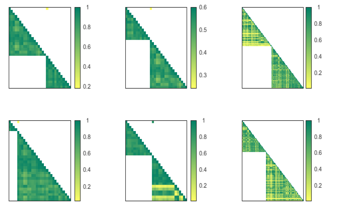
The lower limit of the intra-class correlation λ is set at 0.54, and the upper limit of the inter-class correlation η is set at 0.50. In the solving of this paper, the CPU used is Intel i9-13900K 5.80GHz and the RAM is VENGEANCE DDR5 96GB 4800MHz. In this example, solving DRMBIP-p and DRMBIP-v took 145.01 seconds and 50.68 seconds, respectively. The results are shown in Table 2. And the visualization results are shown in Figure 1.
Table 2. Evaluation indexes for dimensionality reduction algorithms.
Case 1 Case 2 Case 3 Case 4 Case 5
Index1 0.6018 0.6018 0.5210 0.0090 0.0033
Index2 0.8528 0.8106 0.7893 0.1345 0.0394
Index3 0.6669 0.6669 0.6552 0.3578 0.0226
Index4 0.9086 0.9112 0.8596 0.8033 0.6845
Index5 0.6669 0.6669 0.6552 0.3578 0.0226
Index7 0.1791 0.2807 0.0184 0.8381 0.3279
Index8 0.1791 0.2807 0.0184 0.8381 0.3279
Compactness 1.0282 0.9973 1.2433 1.2396 1.6834
Separation 2.6867 2.6207 2.6634 1.3752 2.3058
DVI 0.8184 0.8184 0.6449 0.3313 0.2488
SI 0.5095 0.5095 0.5472 0.2300 0.1721
DBI 0.7684 0.7577 0.7680 1.8128 1.4645
Figure 1. Indicator Relationship Map.
In terms of indicator filtering effect, comparing Case 2 with Case 5, the K-Means algorithm with indicator filtering gets better dimensionality reduction effect. Its performance on the evaluation indicators is better than the K-Means algorithm without indicator filtering. However, in the comparison between Case 4 and Case 5, the K-Means algorithm with indicator filtering performs generally on the four indexes involving inter-class distances but performs better on all other indexes.
In terms of dimensionality reduction effect, comparing Case 1 with Case 2, the DRMBIP-p filtered indexes performed better. Only Index4 is inferior, but it also reaches 0.9086. This indicates a very high compactness between classes and a high substitutability of intra-class indicators. Case 3 shows the evaluation results corresponding to DRMBIP-v. Only the compactness is slightly lower than Case 4 among all 12 indexes, and DRMBIP-v performs extremely well.
Comparing Case 1 and Case 3, it is not difficult to find that DRMBIP-p performs better in the evaluation index of intra-class correlation. But there is a huge gap between DRMBIP-v and DRMBIP-p in terms of inter-class correlation, which is due to the pursuit of compactness and separation at the same time in DRMBIP-v.
Comparing the three subfigures in the first row of Figure 1, it is easy to find that the dimensionality reduction results of DRMBIP-p have smaller inter-class correlation and larger intra-class correlation than the K-Means dimensionality reduction results after the indicator filter, and the effect is better. Unlike DRMBIP-p, DRMBIP-v must maximize intra-class correlation and minimize inter-class correlation when performing indicator filtering. As a result, the filtered set of indicators has extremely strong class characteristics. This leads to errors in that classes contain indicators with low correlation in the K-Means algorithm.
In summary, DRMBIP obtains good results. DRMBIP-p adopts the form of parameter to set the lower limit of intra-class correlation and the upper limit of inter-class correlation. It makes the indicator filtering more flexible, and the selected indicators have better compatibility with other algorithms. On the other hand, DRMBIP-v variables are the lower and upper limit parameters of DRMBIP-p. It makes the results of DRMBIP-v more extreme, sacrificing the compatibility with other models in exchange for more obvious class characteristics.

4.2.2 Aspects of the life expectancy

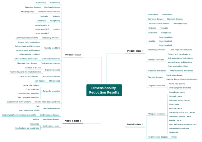
Among the 141 factors affecting life expectancy, diseases account for 130 indicators, most of which are subdivided into subcategories. After filtering and dimensionality reduction of the indicators, the dimensionality can be further reduced by combining these actual categorizations. To facilitate the analysis, we draw the results of the dimensionality reduction of DRMBIP-p and DRMBIP-v in a corresponding mind map, as shown in Figure 2 below.
Figure 2. Structure of the main factors influencing life expectancy.
The dimensionality reduction results of DRMBIP include subcategories such as tuberculosis, diarrhoeal diseases, hepatitis, digestive diseases, neonatal conditions, and congenital anomalies. In addition, the four subcategories of hepatitis, digestive diseases, neonatal conditions, and congenital anomalies include several diseases with high correlation among the diseases, which may share common predisposing factors and require further traceability. Compared to DRMBIP-v, DRMBIP-p lacked diseases in the categories of genitourinary diseases, skin diseases, sudden infant death syndrome, unintentional injuries, and respiratory diseases. In DRMBIP-v, minimizing the inter-class correlation eliminated these diseases that were not highly correlated with the best class centers, resulting in a more pronounced distinction between classes. These diseases with different class characteristics may not have common causative factors and therefore require separate focus. In contrast, DRMBIP-v is built with more relaxed parameters to find the best indicators while maintaining inter-class and intra-class correlation thresholds. Compared with DRMBIP-p, DRMBIP-v does not include malignant neoplasms, which also indicates that there are some common factors among the different causes of malignant neoplasms. But these causative factors are still quite different from each other, and these common factors should be explored, while the factors inducing different types of malignant neoplasms should be studied separately. Similarly, cardiovascular diseases selected only the disease of stroke in DRMBIP-p. However, it selected two diseases that belonged to two categories in DRMBIP-v. It indicated that there were more complex causative factors in cardiovascular diseases and that it was difficult to find the causes of cardiovascular diseases, which should be monitored separately to find out the causes of the diseases respectively.
Analysis of the 30 indicators analyzed reveals several key factors that influence life expectancy. We have summarized the areas on which countries at all stages of development should focus, in the hope of maximizing the efficiency of the use of health resources and improving life expectancy for all.
(1) Strengthening drinking water sanitation
Many infectious diseases can be transmitted through the digestive tract, such as hepatitis and diarrhoeal diseases, and protecting water sources is tantamount to blocking the transmission of viruses. In 2016, an outbreak of acute jaundice hepatitis occurred in Chad, Africa, where unsafe water use led to the widespread spread of the disease. Countries should improve the safety of water sources to fundamentally disrupt the transmission of such infectious diseases.
(2) Strengthening the control of food additives
At present, many countries do not pay enough attention to food safety. For example, the artificial sweetener aspartame, which was first classified as “possibly carcinogenic to humans” in July this year, is now widely used by the food industry in various countries. Currently, many countries have lax control over food additives, leading to excessive intake by consumers and resulting in an increase in the prevalence of digestive diseases and cancers every year.
(3) Enactment of the early pregnancy screening policy
Conservative estimates put the global average incidence of malformed fetuses at 2%-3%, with the incidence of severely malformed fetuses at 0.5%-1%. For high-risk pregnant women with a family history of serious genetic defects, infectious diseases in early pregnancy, alcohol, drug addiction, those who have received radiation therapy, as well as those who are malnourished and weak, the risk of malformed fetuses will be even higher. And these high-risk pregnant women should be screened as much as possible.

5 Conclusion

In this paper, we propose two DRMBIP to find the most dominant geometric structures from high-dimensional complex data and reveal their influence patterns. Taking the life expectancy data of 184 countries in the world as an example, we calculate the correlation between 141 relevant disease indicators and use DRMBIP to eliminate abnormal indicators and filter indicators. We find 30 important factors affecting life expectancy. It automatically clustered into the optimal two classes based on the correlation. Taking the central indicators of each class as the starting point, we analyzed the correlation indicators and disease categories. We found that there are four main categories of disease factors affecting life expectancy, namely hepatitis, digestive diseases, congenital anomalies, and malignant neoplasms.
We compare the effect of the proposed model with the traditional K-Means algorithm on indicator dimensionality reduction, and find that the algorithm in this paper has the following advantages:
(1) More interpretable
The class center, as an important entry point for clustering analysis, should have strong interpretability. When traditional clustering algorithms are used for indicator dimensionality reduction, the class center is not real, from the virtual class center into the analysis may lead to a certain bias. The models proposed in this paper are based on dimensionality reduction on the factors affecting life expectancy, and the class center indicators affecting life expectancy are obtained. DRMBIP-p: preterm birth complications; trachea, bronchus, lung cancers. DRMBIP-v: cardiomyopathy, myocarditis, endocarditis; other congenital anomalies. From the center of the class, we mined out the three most likely common influences and gave suggestions for prevention and control.
(2) No need to consider the number of clusters
In the traditional clustering model, some models use the number of clusters as a parameter, and the number of clusters seriously affects the model. To obtain the best result, it is necessary to consider the factors such as the compactness and the separation. And it needs to test the parameter to choose the best value in the set of the number of clusters. DRMBIP variables the parameter number of clusters, so the model can find the number of clusters with the best clustering effect. In selecting the 30 important indicators influencing life expectancy, the optimal number of clusters can be found. Eventually, the relevant indicators were classified into two classes with obvious class characteristics.
(3) Automatic elimination of abnormal indicators
There are many indicators that are difficult to classify, and it is not appropriate to force them into a particular class. By analyzing the relevant indicators affecting life expectancy, we found that the average value of the correlation is 0.4693. It indicates that many indicators are difficult to classify and are in low-density areas in the indicator space. To select the important factors from the indicators affecting life expectancy, this paper sets the number of class centers as 30. It obtains better results which not only shows excellent clustering and dimensionality reduction effect, but also provides a compatible low-dimensional indicator system for other clustering models.
(4) Easier to view results
In multidimensional data, the geometric structure between data is often difficult to display in the two-dimensional plane. DRMBIP adopts correlation to measure the distance between indicators, it makes the visualization display easy. We can mine the main geometric structures and special details in the intra-class and inter-class indicators based on the indicator relationship maps of the 30 important indicators.
At present, the research on DRMBIP is still in the exploratory stage. In the future, we will further validate the dimensionality reduction effect under different sizes of datasets. At the same time, we will develop parallel dimensionality reduction algorithms under big data. Eventually, a complete set of accurate dimensionality reduction algorithms for big data will be formed for data mining personnel.

Acknowledgements

The authors thank anonymous peer reviewers for improving the paper.

Author contributions

Wei Cui (Email: cuiwei@imut.edu.cn) optimized the models and wrote the paper. Ren Mu (Email: muren@imut.edu.cn) initiated the idea and built the originally models. Zhiqiang Xu (17607156506@163.com) processed the data and did experiments.

Conflict of interest statement

The authors declare no competing interests.

Funding information

This work was supported by the National Natural Science Foundation of China (Nos. 72371115), the Natural Science Foundation of Jilin, China (No. 20230101184JC).

Data availability

All the data we used in this paper are publicly available and can be downloaded from the official website of the World Health Organization.
[1]
Abdi, H., & Williams, L. J. (2010). Principal component analysis. Wiley interdisciplinary reviews: computational statistics, 2(4), 433-459.

DOI

[2]
Achterberg, T., Bixby, R. E., Gu, Z., Rothberg, E., & Weninger, D. (2020). Presolve reductions in mixed integer programming. INFORMS Journal on Computing, 32(2), 473-506.

DOI

[3]
Alexiou, A., Mason, K., Fahy, K., Taylor-Robinson, D., & Barr, B. (2021). Assessing the impact of funding cuts to local housing services on drug and alcohol related mortality: a longitudinal study using area-level data in England. International Journal of Housing Policy, 1-19.

[4]
Baumann, F. (2021). The next frontier—human development and the anthropocene:UNDP human development report 2020. Environment: Science and Policy for Sustainable Development, 63(3), 34-40.

[5]
Bayati, M., Noroozi, R., Ghanbari-Jahromi, M., & Jalali, F. S. (2022). Inequality in the distribution of Covid-19 vaccine: a systematic review. International journal for equity in health, 21(1), 1-9.

DOI

[6]
Belkin, M., & Niyogi, P. (2001). Laplacian eigenmaps and spectral techniques for embedding and clustering. Advances in neural information processing systems, 14.

[7]
Bhadra, A., Datta, J., Polson, N. G., & Willard, B. (2019). Lasso meets horseshoe. Statistical Science, 34(3), 405-427.

[8]
Can-can, Y., Shuai, T., Shan, T., & Wen-tao, Z. (2022). UMAP-Assisted Fuzzy C-Clustering Method for Recognition of Terahertz Spectrum. Spectroscopy and Spectral Analysis, 42(9), 2694-2701.

[9]
Cortés, P., Muñuzuri, J., Onieva, L., & Guadix, J. (2018). A discrete particle swarm optimisation algorithm to operate distributed energy generation networks efficiently. International Journal of Bio-Inspired Computation, 12(4), 226-235.

DOI

[10]
Currie, J., Boyce, T., Evans, L., Luker, M., Senior, S., Hartt, M.,... Humphreys, C. (2021). Life expectancy inequalities in Wales before COVID-19: an exploration of current contributions by age and cause of death and changes between 2002 and 2018. Public Health, 193, 48-56.

DOI PMID

[11]
Deutelmoser, H., Scherer, D., Brenner, H., Waldenberger, M., Study, I., Suhre, K.,... Lorenzo Bermejo, J. (2021). Robust Huber-LASSO for improved prediction of protein, metabolite and gene expression levels relying on individual genotype data. Briefings in Bioinformatics, 22(4), bbaa230.

[12]
Ding, C., & He, X. F. (2004). K-means clustering via principal component analysis. Paper presented at the Proceedings of the twenty-first international conference on Machine learning.

[13]
Espadoto, M., Martins, R. M., Kerren, A., Hirata, N. S., & Telea, A. C. (2019). Toward a quantitative survey of dimension reduction techniques. IEEE transactions on visualization and computer graphics, 27(3), 2153-2173.

DOI

[14]
Ezugwu, A. E., Ikotun, A. M., Oyelade, O. O., Abualigah, L., Agushaka, J. O., Eke, C. I.,... Akinyelu, A. A. (2022). A comprehensive survey of clustering algorithms: State-of-the-art machine learning applications, taxonomy, challenges, and future research prospects. Engineering Applications of Artificial Intelligence, 110, 104743.

DOI

[15]
Fahim, A. (2023). Adaptive Density-Based Spatial Clustering of Applications with Noise (ADBSCAN) for Clusters of Different Densities. Computers, Materials & Continua, 75(2), 3695-3712.

[16]
Farhud, D. D. (2022). Hypothetical Strategies of Gene and Environmental Influence on Life Expectancy: A Brief Review. Iranian Journal of Public Health, 51(11), 2382.

[17]
Flegner, P., Kačur, J., Frančáková, R., Durdán, M., & Laciak, M. (2023). Application of Cluster Analysis for Classification of Vibration Signals from Drilling Stand Aggregates. Applied Sciences, 13(10), 6337.

[18]
Golalipour, K., Akbari, E., Hamidi, S. S., Lee, M., & Enayatifar, R. (2021). From clustering to clustering ensemble selection: A review. Engineering Applications of Artificial Intelligence, 104, 104388.

DOI

[19]
Guha, S., Rastogi, R., & Shim, K. (2000). ROCK: A robust clustering algorithm for categorical attributes. Information systems, 25(5), 345-366.

DOI

[20]
Gupta, S., Zhang, Y., & Su, R. (2022). Urban traffic light scheduling for pedestrian-vehicle mixed-flow networks using discrete sine-cosine algorithm and its variants. Applied Soft Computing, 120, 108656.

DOI

[21]
Jia, W. K., Sun, M. L., Lian, J., & Hou, S. J. (2022). Feature dimensionality reduction: a review. Complex & Intelligent Systems, 8(3), 2663-2693.

[22]
Kruskal, J. B., & Wish, M. (1978). Multidimensional scaling: Sage.

[23]
Lee, D. D., & Seung, H. S. (1999). Learning the parts of objects by non-negative matrix factorization. Nature, 401(6755), 788-791.

DOI

[24]
Li, X. D., Sun, D. F., & Toh, K. C. (2020). An asymptotically superlinearly convergent semismooth Newton augmented Lagrangian method for linear programming. SIAM Journal on Optimization, 30(3), 2410-2440.

DOI

[25]
Lichtenberg, F. R. (2022). The effect of pharmaceutical innovation on longevity: Evidence from the US and 26 high-income countries. Economics & Human Biology, 46, 101124.

[26]
Liu, W. H., Zeng, S., Wu, G. J., Li, H., & Chen, F. F. (2021). Rice seed purity identification technology using hyperspectral image with LASSO logistic regression model. Sensors, 21(13), 4384.

[27]
McInnes, L., Healy, J., & Melville, J. (2018). Umap: Uniform manifold approximation and projection for dimension reduction. arXiv preprint arXiv:1802.03426.

[28]
Nasiri, E., Berahmand, K., Rostami, M., & Dabiri, M. (2021). A novel link prediction algorithm for protein-protein interaction networks by attributed graph embedding. Computers in Biology and Medicine, 137, 104772.

DOI

[29]
Oyewole, G. J., & Thopil, G. A. (2023). Data clustering: Application and trends. Artificial Intelligence Review, 56(7), 6439-6475.

DOI

[30]
Rani, R., Khurana, M., Kumar, A., & Kumar, N. (2022). Big data dimensionality reduction techniques in IoT: Review, applications and open research challenges. Cluster Computing, 25(6), 4027-4049.

DOI

[31]
Roweis, S. T., & Saul, L. K. (2000). Nonlinear dimensionality reduction by locally linear embedding. science, 290(5500), 2323-2326.

DOI PMID

[32]
Roy, S., Howlader, J., & Sanyal, G. (2022). A novel approach of data hiding in video using region selection and PCA. Multimedia Tools and Applications, 81(10), 14553-14571.

DOI

[33]
Sawant, M., & Bhurchandi, K. M. (2022). Discriminative aging subspace learning for age estimation. Soft Computing, 26(18), 9189-9198.

DOI

[34]
Sen, A. (1998). Mortality as an indicator of economic success and failure. The economic journal, 108(446), 1-25.

[35]
Shuai, Y. (2022). A Full-Sample Clustering Model Considering Whole Process Optimization of Data. Big Data Research, 28, 100301.

DOI

[36]
Song, X., Li, S. H., Qi, Z. Q., & Zhu, J. L. (2022). A spectral clustering algorithm based on attribute fluctuation and density peaks clustering algorithm. Applied Intelligence, 1-15.

[37]
Stephenson, W. (1935). Technique of factor analysis. Nature, 136(3434), 297.

[38]
Tenenbaum, J. B., Silva, V. D., & Langford, J. C. (2000). A global geometric framework for nonlinear dimensionality reduction. science, 290(5500), 2319-2323.

DOI PMID

[39]
Tian, P., Shen, H., & Abolfathi, A. (2022). Towards Efficient Ensemble Hierarchical Clustering with MapReduce-based Clusters Clustering Technique and the Innovative Similarity Criterion. Journal of Grid Computing, 20(4), 34.

[40]
Ullah, B., Kamran, M., & Rui, Y. (2022). Predictive modeling of short-term rockburst for the stability of subsurface structures using machine learning approaches: T-SNE, K-Means clustering and XGBoost. Mathematics, 10(3), 449.

[41]
Van der Maaten, L., & Hinton, G. (2008). Visualizing data using t-SNE. Journal of machine learning research, 9(11).

[42]
Vaswani, A., Shazeer, N., Parmar, N., Uszkoreit, J., Jones, L., Gomez, A. N.,... Polosukhin, I. (2017). Attention is all you need. Advances in neural information processing systems, 30.

[43]
Wang, S. L., Li, Q., Zhao, C. F., Zhu, X. G., Yuan, H. N, & Dai, T. R. (2021). Extreme clustering-a clustering method via density extreme points. Information Sciences, 542, 24-39.

DOI

[44]
Xia, J. Z., Zhang, Y. C., Song, J., Chen, Y., Wang, Y. H., & Liu, S. (2021). Revisiting dimensionality reduction techniques for visual cluster analysis: an empirical study. IEEE Transactions on Visualization and Computer Graphics, 28(1), 529-539.

DOI

[45]
Yang, L. J., Yan, L. L., Yang, X. H., Xin, X., & Xue, L. G. (2022). Bayesian nonnegative matrix factorization in an incremental manner for data representation. Applied Intelligence, 1-18.

[46]
Yang, Q., Yin, S. H., Li, Q. P, & Li, Y. P. (2022). Analysis of electricity consumption behaviors based on principal component analysis and density peak clustering. Concurrency and Computation: Practice and Experience, 34(21), e7126.

[47]
Yao, Y. Q., Meng, H., Gao, Y., Long, Z. G., & Li, T. R. (2023). Linear dimensionality reduction method based on topological properties. Information Sciences, 624, 493-511.

DOI

[48]
Yunita, A., Santoso, H. B., & Hasibuan, Z. A. (2022). ‘Everything is data’: towards one big data ecosystem using multiple sources of data on higher education in Indonesia. Journal of Big Data, 9(1), 1-22.

DOI

[49]
Zhang, N., Tian, Y., Wang, X. W., Xu, Y., Zhu, Q. X., & He, Y. L. (2023). Novel Bootstrap-Based Discriminant NPE Integrated With Orthogonal LPP for Fault Diagnosis. IEEE Transactions on Instrumentation and Measurement, 72, 1-9.

[50]
Boutsidis, C., Zouzias, A., Mahoney, M. W., & Drineas, P. (2014). Randomized dimensionality reduction for k-means clustering. IEEE Transactions on Information Theory, 61(2), 1045-1062.

DOI

[51]
Maldonado, S., Carrizosa, E., & Weber, R. (2015). Kernel penalized k-means: A feature selection method based on kernel k-means. Information sciences, 322, 150-160.

DOI

Outlines

/

京ICP备05002861号-43

Copyright © 2023 All rights reserved Journal of Data and Information Science

E-mail: jdis@mail.las.ac.cn Add:No.33, Beisihuan Xilu, Haidian District, Beijing 100190, China

Support by Beijing Magtech Co.ltd E-mail: support@magtech.com.cn