Research Papers

A comparison of model choice strategies for logistic regression

  • Markku Karhunen ,
Expand
  • Built Environment Solutions unit, Finnish Environment Institute (Syke), Latokartanonkaari 11, 00790 Helsinki, Finland
†Markku Karhunen (Email: ; ORCID: 0000-0001-9086-8214).

Received date: 2023-10-11

  Revised date: 2023-12-04

  Accepted date: 2023-12-22

  Online published: 2024-01-24

Abstract

Purpose: The purpose of this study is to develop and compare model choice strategies in context of logistic regression. Model choice means the choice of the covariates to be included in the model.

Design/methodology/approach: The study is based on Monte Carlo simulations. The methods are compared in terms of three measures of accuracy: specificity and two kinds of sensitivity. A loss function combining sensitivity and specificity is introduced and used for a final comparison.

Findings: The choice of method depends on how much the users emphasize sensitivity against specificity. It also depends on the sample size. For a typical logistic regression setting with a moderate sample size and a small to moderate effect size, either BIC, BICc or Lasso seems to be optimal.

Research limitations: Numerical simulations cannot cover the whole range of data-generating processes occurring with real-world data. Thus, more simulations are needed.

Practical implications: Researchers can refer to these results if they believe that their data-generating process is somewhat similar to some of the scenarios presented in this paper. Alternatively, they could run their own simulations and calculate the loss function.

Originality/value: This is a systematic comparison of model choice algorithms and heuristics in context of logistic regression. The distinction between two types of sensitivity and a comparison based on a loss function are methodological novelties.

Cite this article

Markku Karhunen . A comparison of model choice strategies for logistic regression[J]. Journal of Data and Information Science, 2024 , 9(1) : 37 -52 . DOI: 10.2478/jdis-2024-0001

1 Introduction

Model choice, i.e., the choice of covariates to be included in a model, is a lasting problem in statistics. Numerous solutions have been proposed. Among them, one of the oldest and most widely known is the Akaike’s information criterion (AIC) (Akaike, 1973). Bayesian information criterion (BIC) (Schwarz, 1978) is also widely used. They are target functions which are minimized to arrive at a favorable model. AIC aims to choose the model which has the best predictive power and BIC aims to choose the true model if it is included in the tested subset. BIC is more conservative than AIC, as it penalizes each additional parameter more strictly, and thus, BIC favors smaller models. However, as the derivations of AIC and BIC are based on asymptotic arguments (Akaike, 1973; Schwarz, 1978), it makes sense to compare their performance in finite data sets.
Regularized regression models offer another approach to the model choice problem. These are regression models where the model fit is penalized by some norm of the parameter vector. Methods based on the L1 norm, most notably Lasso (Tibshirani, 1996) and Adaptive Lasso (Zou, 2006) produce a model where a parsimonious subset of the available covariates is used, and thus, they perform model choice. However, regularized regressions based on the L2 norm (Hoerl & Kennard, 1970) assign a small contribution to all variables, and thus, they do not perform model choice.
Logistic regression models are models for binary or binomial outcomes. They are a type of generalized linear model (McCullagh & Nelder, 1989) and perhaps the most widely used of them all. They are frequently used in areas as diverse as genetics (Ayers & Cordell, 2010), clinical medicine (Zhang et al., 2017), econometrics (Karhunen, 2019), consumer research (Bejaei et al., 2015) and environmental science (Saha & Pal, 2019), to name a few. Thus, it is important to study the model choice problem in the context of logistic regression. This paper uses simulated data to compare the performance of nine model choice algorithms. The results show that there is no one-size-fits-all solution.
The rest of this paper is organized as follows. First, the methods to be compared are introduced, then the data generation and then the measures of accuracy (specificity and two different kinds of sensitivity). In the Results section, the accuracy of the different model choice strategies is first discussed, and then the optimal model choice. A discussion concludes.

2 Material and methods

2.1 Methods compared

The logistic regression is here defined without loss of generality for a binary response variable. Formulations where each observational unit is a binomial trial are sometimes seen (e.g., Qian & Field, 2002). However, they can be trivially transformed into the present definition. The logistic regression can be defined through the log-likelihood function
$\begin{aligned} \log L(\boldsymbol{\beta}) & =\sum_{i=1}^{n}\left\{y_{i} \log \left(\frac{1}{1+\exp \left(-\boldsymbol{x}_{i}{ }^{\prime} \boldsymbol{\beta}\right)}\right)+\left(1-y_{i}\right) \log \left(1-\frac{1}{1+\exp \left(-\boldsymbol{x}_{i}{ }^{\prime} \boldsymbol{\beta}\right)}\right)\right\} \\ & =\sum_{i=1}^{n}\left\{y_{i} \boldsymbol{x}_{i}{ }^{\prime} \boldsymbol{\beta}-\log \left(1+\exp \left(\boldsymbol{x}_{i}{ }^{\prime} \boldsymbol{\beta}\right)\right)\right\} \end{aligned}$
where yi∈{0,1} is the dichotomous response, xi is the vector of covariates (involving 1 for the constant term) and β=(βj) denotes the parameter vector, with β1 being the constant term. Below, $\hat{\beta}_{j}$ denotes the maximum-likelihood estimate of βj. Model choice can be understood so that all models are thought to be nested in a ‘full’ model, and various combinations of $\hat{\beta}_{j}$=0 indicate various sub-models. Below, k denotes the dimensionality of the model, i.e., the number of non-zero components in $\hat{\beta}_{j}$.
The following methods are tested for their potential to detect the true model in simulated data:
1. Wald’s tests. This is a one-step procedure where all variables which are univariately significant with P values <0.05 are included in the final model specification. The statistical significance is calculated by using the Wald’s test (e.g., Buse, 1982).
2. Likelihood-ratio test. Let l be the maximized log-likelihood of some non-empty model and l0 be the maximized log-likelihood of the empty model (a model including only the intercept). Under the null hypothesis of no true effect,
LR=2l-2l0
is asymptotically distributed as a chi-squared random variable with k-1 degrees of freedom (e.g., Buse, 1982). Thus, it is possible to calculate a joint P value for each model. This is used as a model choice criterion according to the following rule: i) Calculate a P value for all non-empty models. ii) If some P values are <0.05, choose the model with the smallest P value. iii) If all P values are ≥0.05, choose the empty model. Notably, it can be shown that this leads to a model choice criterion which is concave in k.
3. Akaike’s AIC (1973). The model with the minimal
AIC=-2l+2k
is chosen.
4. Schwarz’s BIC (1978). The model with the minimal
BIC=-2l+log(n)k
is chosen.
5. AICc of Hurvich and Tsai (1989). The idea of this method is to correct for the fact that AIC has been derived assuming infinite data sets. Thus, the criterion to be minimized is
$A I C c=-2 l+2 k \frac{n}{n-k-2}$
AICc as BICc below (McQuarrie, 1999) has been derived for the Gaussian regression model. There is a corrected AIC for generalized linear models (Imori et al., 2014) but it was found too slow for the Monte Carlo simulations of this study.
6. BICc of McQuarrie (1999). The idea is to correct for the finite-sample bias of BIC. The model with the minimal
$B I C c=-2 l+\log (n) k \frac{n}{n-k-2}$
is chosen.
7. MDL of Zhou et al. (2005). This formula was derived from Rissanen’s minimum description length principle (1978) by Qian and Field (2002) following Qian and Künsch (1998). The model with the minimal
$M D L=-2 l+\log \operatorname{det}\left(\mathbf{X}^{\prime} \mathbf{S X}\right)+2 \sum_{j=2}^{k} \log \left|\hat{\beta}_{j}\right|$
is chosen where X is the matrix of covariates, S is a diagonal matrix with $s_{i i}=\hat{p}_{i}\left(1-\hat{p}_{i}\right)$ and $\hat{p}_{i} \in(0,1)$ is the model prediction for observation i.
Note that the sums ranging from 2 to k involve the regression coefficients, disincluding the constant term β1.
8. Tibshirani’s Lasso (1996). A model with all covariates is fitted, but instead of maximizing the log-likelihood, one maximizes
$F_{1}=\log L(\boldsymbol{\beta})-\lambda \sum_{j=2}^{k}\left|\beta_{j}\right|$
where λ>0 is a parameter to be chosen by cross validation. The maximization of F1 can produce a parsimonious solution, i.e., one with βj=0, and thus, Lasso performs model choice (Tibshirani, 1996). We use the R package glmnet (Friedman et al., 2010; Tay et al., 2023) to fit Lasso. In cross validation, we use mean-square error (MSE) to determine λ.
9. Zou’s Adaptive Lasso (2006). Otherwise the same as Lasso, but the target function to be maximized is
$F_{2}=\log L(\boldsymbol{\beta})-\lambda \sum_{j=2}^{k} \frac{\left|\beta_{j}\right|}{\left|b_{j}\right|^{\gamma}}$
where γ>0 and bj is some statistically consistent estimate of βj. Here, we choose γ=0.5 and use the maximum-likelihood estimate as bj. We choose λ by cross validation (minimizing MSE) and use glmnet (Friedman et al., 2010; Tay et al., 2023) to fit Adaptive Lasso.
In this study, methods 2-7 are applied so that all models are scored with each respective information criterion. This is contrary to the practice of stepwise model selection but is appropriate for a small number of covariates.

2.2 Test data

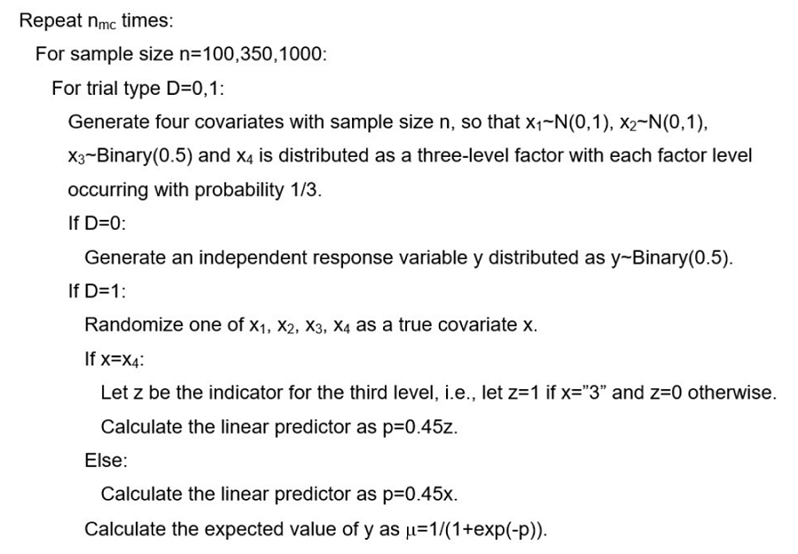
Test data were used to compare the performance of different model choice algorithms. The data were generated by using Algorithm 1. Variations of Algorithm 1 are used in the Appendix to generate three additional scenarios: One with two true effects for each data of type D=1, one where the effect size is larger (β=1.35) and one where the logistic model is misspecified.
Algorithm 1
In Algorithm 1, β=0.45 was chosen as the effect size, as it produces Pearson’s product moment correlation 0.11 for the binary covariate, which in turn can be interpreted as a small effect size (Cohen, 1988).

2.3 Measures of accuracy

For each model choice algorithm, three measures of accuracy were calculated, i.e., specificity, sensitivity-1 and sensitivity-2. Specificity was defined as
$\text { Spec }=\frac{\text { no. of empty models chosen for data type } D=0}{n_{m c}}$
Sensitivity-1 was defined as
$\text { Sens } 1=\frac{\text { no. of models with only covariate } \mathrm{x} \text { chosen for data type } \mathrm{D}=1}{\mathrm{n}_{\mathrm{mc}}}$
where x denotes the true covariate used to generate data according to Algorithm 2. Sensitivity-2 was defined as
$\text { Sens } 2=\frac{\text { no. of models with covariate } x \text { chosen for data type } D=1}{n_{m c}}$
Thus, Sens2≥Sens1 always, as the criterion involved in calculating Sensitivity-2 is easier to satisfy. Sensitivity-1 measures the methods’ ability to detect a true non-empty model, whereas sensitivity-2 measures their ability to detect a true covariate at the cost of including noise covariates in the model. Additionally, a loss function was defined as
Loss=1-Spec+ϕ(1-Sens2)
with ϕ>0 denoting the relative weight given to false negatives, i.e., failures to observe true effects.

3 Results

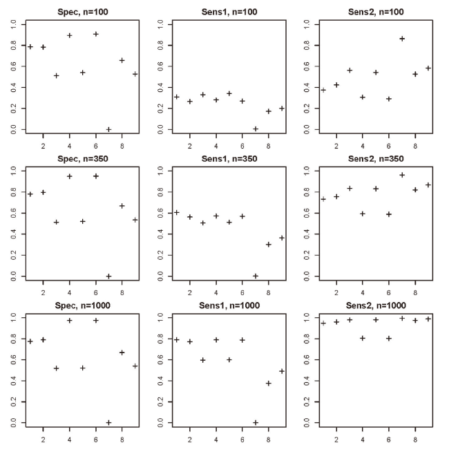
The main model comparison was run by using Algorithm 1 with nmc=10,000. Figure 1 and Table 1 present the results. The following observations can be made: Both Wald’s tests and likelihood-ratio test have reasonably high accuracy in these data. AIC, AICc, Lasso and Adaptive Lasso have low specificity and high sensitivity-2. BIC and BICc have high specificity and with larger sample sizes (n=350 and n=1,000), they also outperform the AIC-based methods in terms of sensitivity-1 because their stronger dimensional penalties help to avoid the inclusion of noise covariates in the model. The differences between AIC and AICc (or BIC and BICc) are barely visible. MDL has such low specificity that it is not useful in these data.
Figure 1. Comparison of model comparison methods. The methods tried are 1. Wald’s tests, 2. likelihood-ratio test, 3. AIC, 4. BIC, 5. AICc, 6. BICc, 7. MDL, 8. Lasso and 9. Adaptive Lasso. The sampling variation is minimal in this image, with confidence intervals smaller than the crosses. For distinction of sensitivity-1 and sensitivity-2, see Methods.
Table 1. Results of the main model comparison.
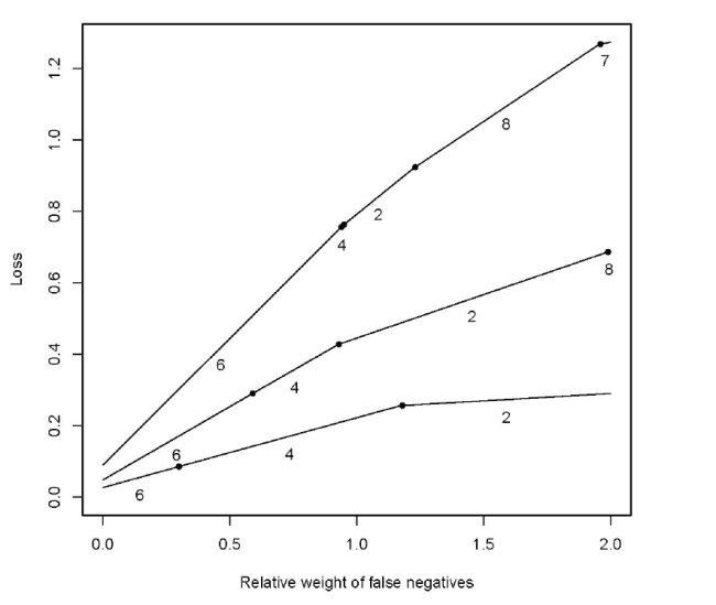
There is always a trade-off between sensitivity and specificity. In this study, sensitivity-2 goes theoretically to 1.00 when specificity goes to 0.00, and vice versa. These extreme values can be produced by choosing always an empty model or always including all covariates in the model. It depends on the preferences of each research team how to tackle this trade-off. Figure 2 illustrates the dilemma. It shows the efficient frontier of the loss function defined in Methods. E.g., for ϕ=0.50 and n=100, BICc is the optimal method. If the researchers are apprehensive to report false positives, they are on the left-hand side of the figure. On the other hand, if they believe that they need to capture all plausible effects in the model, they are more on the right.
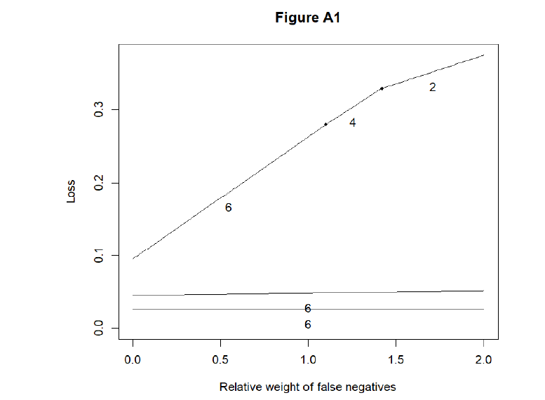
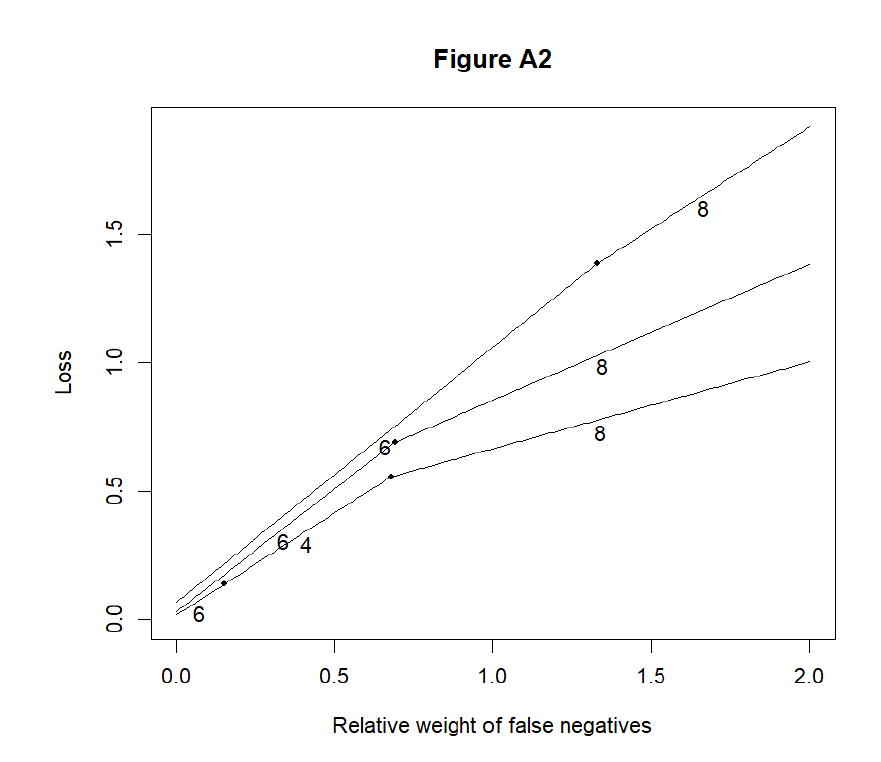
Figure 2. Optimal methods. x axis is the relative weight of type II errors (failures to detect true covariates). The weight of type I errors (choosing noise covariates) is set to one. The highest curve corresponds to n=100, whereas the middle curve and the lowest curve correspond to n=350 and n=1,000, respectively. The numbers under the line segments indicate the optimal methods.
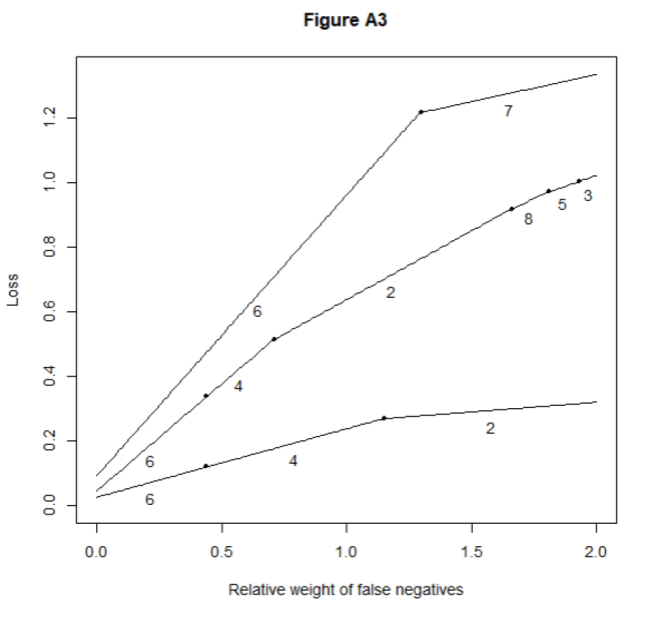
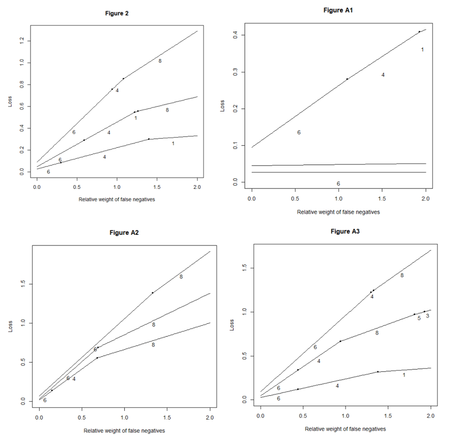
The Appendix of this paper presents three alternative scenarios: One with a larger effect size, one with two effects and one with a misspecified model structure. As was expected, the stronger the effect, the easier it is to detect. Thus, in the strong effect’s scenario, all methods have a high sensitivity-2. In the two effects’ scenario, the two effects are confounded by each other. In this case, the sensitivities of all methods severely fall. The same applies to a lesser degree on the misspecified model’s scenario. However, the big picture as measured by the choice of optimal model (Figure 2) changes surprisingly little. In all these scenarios, a conservative researcher should choose BIC or BICc and only after some ϕ≈1.0, something else should be used. The other method of choice is either likelihood ratio test or Lasso. The only exception to this pattern is the strong effect’s scenario with n=350 and n=1,000. In these data, BICc is optimal for all ϕ because Sens2=1.00. However, it may be argued that researchers would be lucky to have effects and sample sizes this large simultaneously.
Finally, likelihood ratio test and MDL were removed from the comparison because of their weird behavior in some of the scenarios and Figure 2 was re-run (see Appendix). In this analysis, the take-home message is to use BIC or BICc for a low ϕ and Wald’s tests or Lasso for a larger ϕ.

4 Discussion

This paper has presented a systematic comparison of nine model choice algorithms for use with logistic regression models. Out of the methods presented, four are information criteria (AIC, BIC, AICc and BICc), two are regularized regressions (Lasso and Adaptive Lasso) and two are based on commonly used statistical tests (Wald’s tests and the likelihood-ratio test). Even though derived from different principles, MDL is used similarly to the information criteria, i.e., it is a target function to be minimized.
Wald’s tests are not strictly speaking a model choice method, but a heuristic to construct a single model. Likelihood ratio test is typically used to test nested models against each other. In this paper, it is used to score and rank all model variants. This may lead to some strange behaviors as noted in the Appendix. All methods presented here have their respective strengths and weaknesses. Whereas a conservative researcher might prefer BIC or BICc, a more liberally minded one might prefer likelihood-ratio test, Wald’s tests or Lasso. It should be noted that these results concern small model choice problems, i.e., ones with few covariates. When the number of covariates increases, it soon becomes impractical to score all models which limits the accuracy of the information criteria. On the other hand, in massively multivariate data sets, missing values often limit the accuracy of Lasso and Adaptive Lasso. Furthermore, the optimal methods are here calculated on basis of sensitivity-2. If sensitivity-1 is used instead, a different pattern may arise.
There are many developments of Akaike’s original ideas, among them the idea of correcting AIC for small-sample bias (Cavanaugh, 1997; Imori et al., 2014; Sugiura, 1978). Implementing the method of Imori et al. (2014) is left for future work. The extension of this study to other model types, e.g., Gaussian regressions or time-series models, is also left for future work.
Finally, it should be noted that the inclusion of some covariate in a statistical model does not mean that it is significant or that the effect is true. On the contrary, the significance should be assessed based on statistical tests, and ever importantly, the effect size. Thus, the multivariate models produced by model choice algorithms should be regarded only as starting points of long discussions.

Appendix

Alternative scenarios

Stronger effect

In this scenario, Algorithm 1 is run with 𝛽 = 1.35. This produces a product moment correlation of 0.31 between the outcome and the true binary covariate which could still be termed as a moderate effect. The results are presented below. Notably, Sens1 of likelihood ratio test decreases quite rapidly when the sample size is increased, whereas in the main results, Sens1 increases with sample size. This means that likelihood ratio test tends to include too many noise covariates in the model.

Two effects

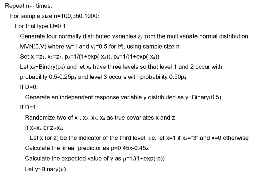
Here, it is assumed that there are two effects with opposite signs and the covariates involving them are positively correlated. Thus, the two effects confound each other and the true model should be more difficult to identify than in the main analysis. Algorithm 1 is modified into Algorithm A1.
Sensitivity-1 and 2 are modified so that it is required that both true effects are detected.
Algorithm A1

Misspecified model

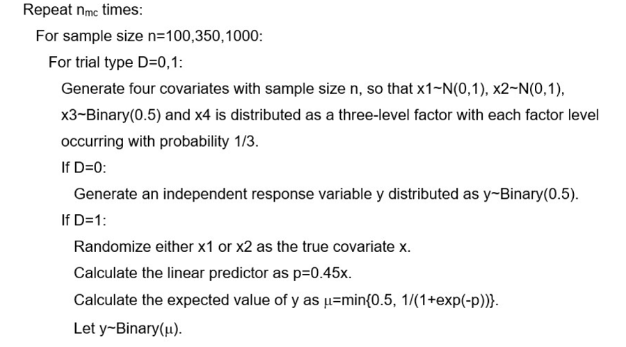
In this scenario, the logistic model is misspecified, as the effect of the true covariate is non-linear. Here, it is assumed that either x1 or x2 is the true covariate (if there is one in the model), as the non-linearity can be defined only for quantitative covariates. Algorithm 1 is modified into Algorithm A2.
Algorithm A2

Re-run without likelihood ratio and MDL

In this analysis, Figure 2 and its counterparts (Figures A1-A3) were run without likelihood ratio test and MDL. The results are as below.
[1]
Akaike, H. (1973). Information theory and an extension of the maximum likelihood principle. In B. N. Petrov, & F. Csaki (Eds.), Proceedings of the Second International Symposium on Information Theory (pp. 267-281). Budapest: Akademiai Kiado.

[2]
Ayers, K. L., & Cordell, H. J. (2010). SNP selection in genome-wide and candidate gene studies via penalized logistic regression. Genetic Epidemiology, 34(8), 879-891.

DOI PMID

[3]
Bejaei, M., Wiseman, K., & Cheng, K. M. (2015). Developing logistic regression models using purchase attributes and demographics to predict the probability of purchases of regular and specialty eggs. British Poultry Science, 56(4), 425-435.

DOI

[4]
Buse, A. (1982). The likelihood ratio, Wald, and Lagrange multiplier tests: An expository note. The American Statistician, 36(3a), 153-157.

[5]
Cavanaugh, J. E. (1997). Unifying the derivations for the Akaike and corrected Akaike information criteria. Statistics & Probability Letters, 33(2), 201-208.

DOI

[6]
Cohen, J. (1988). Statistical Power Analysis for the Behavioral Sciences. (2nd ed). Routledge.

[7]
Friedman, J., Hastie, T., & Tibshirani, R. (2010). Regularization paths for generalized linear models via coordinate descent. Journal of Statistical Software, 33(1), 1.

[8]
Hoerl, A. E., & Kennard, R. W. (1970). Ridge regression: Biased estimation for nonorthogonal problems. Technometrics, 12(1), 55-67.

DOI

[9]
Hurvich, C. M., & Tsai, C-L. (1989). Regression and time series model selection in small samples. Biometrika, 76(2), 297-307.

DOI

[10]
Imori, S., Yanagihara, H., & Wakaki, H. (2014). Simple formula for calculating bias-corrected AIC in generalized linear models. Scandinavian Journal of Statistics, 41(2), 535-555.

DOI

[11]
Karhunen, M. (2019). Algorithmic sign prediction and covariate selection across eleven international stock markets. Expert Systems with Applications, 115, 256-263.

DOI

[12]
McGullagh, P., & Nelder, J. A. (1989). Generalized Linear Models. (2nd ed). Chapman & Hall/CRC.

[13]
McQuarrie, A. D. (1999). A small-sample correction for the Schwarz SIC model selection criterion. Statistics & Probability Letters, 44(1) 79-86.

DOI

[14]
Qian, G. Q., & Field, C. (2002). Using MCMC for logistic regression model selection involving large number of candidate models. In Fang, KT., Niederreiter, H., Hickernell, F.J. (Eds.), Monte Carlo and Quasi-Monte Carlo Methods 2000. Springer, Berlin, Heidelberg.

[15]
Qian, G. Q., & Künsch, H. R. (1998). Some notes on Rissanen’s stochastic complexity. IEEE Transactions on Information Theory, 44(2), 782-786.

DOI

[16]
Rissanen, J. (1978). Modeling by shortest data description. Automatica, 14(5), 465-471.

DOI

[17]
Saha, T. K., & Pal, S. (2019). Exploring physical wetland vulnerability of Atreyee river basin in India and Bangladesh using logistic regression and fuzzy logic approaches. Ecological Indicators, 98, 251-265.

DOI

[18]
Schwarz, G. (1978). Estimating the dimension of a model. The Annals of Statistics, 461-464.

[19]
Sugiura, N. (1978). Further analysis of the data by Akaike’s information criterion and the finite corrections. Communications in Statistics - Theory and Methods, 7(1), 13-26.

[20]
Tay, J. K., Narasimhan, B., & Hastie, T. (2023). Elastic net regularization paths for all generalized linear models. Journal of Statistical Software, 106.

[21]
Tibshirani, R. (1996). Regression shrinkage and selection via the lasso. Journal of the Royal Statistical Society Series B: Statistical Methodology, 58(1), 267-288.

[22]
Zhang, Y. Y., Zhou, X. B., Wang, Q. Z., & Zhu, X. Y. (2017). Quality of reporting of multivariable logistic regression models in Chinese clinical medical journals. Medicine, 96(21).

[23]
Zhou, X. B., Wang, X. D., & Dougherty, E. R. (2005). Gene selection using logistic regressions based on AIC, BIC and MDL criteria. New Mathematics and Natural Computation, 1(01), 129-145.

DOI

[24]
Zou, H. (2006). The adaptive Lasso and its oracle properties. Journal of the American Statistical Association, 101(476), 1418-1429.

DOI

Outlines

/

京ICP备05002861号-43

Copyright © 2023 All rights reserved Journal of Data and Information Science

E-mail: jdis@mail.las.ac.cn Add:No.33, Beisihuan Xilu, Haidian District, Beijing 100190, China

Support by Beijing Magtech Co.ltd E-mail: support@magtech.com.cn