Let G=(V,E) be an undirected network, where V= (v_k)_k=1,…,N denotes the set of nodes or vertices and E denotes the set of links or edges. As collaboration (of scientists, universities, countries), bibliographic coupling (of articles, books), and co-citation (of articles, books) are all examples of undirected networks, it goes without saying that the study of these networks is of great importance for bibliometrics (Rousseau et al., 2018).

We assume that #V = N > 1. A chain in a network is a sequence of different nodes one by one connected by edges. The distance d between two nodes is equal to the number of links situated on a shortest chain (often called a shortest path) between these two nodes. Consequently, the distance between two nodes connected by an edge is equal to one. Each network studied in this article is assumed to be connected, i.e. there is a chain between any two nodes. Hence, for each node, there exists another node at a distance one. The total number of distances between any pair of nodes in this network is equal to N(N-1)/2, where, for v₁,v₂ ∈ V, d(v₁,v₂)=d(v₂,v₁) is considered only once.

Notation. We denote by α_j, j= 1,…, N-1, the number of times distance j occurs in network G. The array A=(α₁, α₂,…,α_N-1) is called the α-array or distance array of the network G.

Some immediate properties

We give a short proof of

Indeed, if $\alpha_{2}>\frac{(N-1)(N-2)}{2}$ then $\frac{N(N-1)}{2}-\sum_{j=1}^{N-1} \alpha_{1} \geq \alpha_{1}+\alpha_{2}>(N-1)+\frac{(N-1)(N-2)}{2}$$\frac{N(N-1)}{2}$, which is a contradiction.

6) In a chain of length j there are 2 chains of length j-1, 3 chains of length j-2, and k chains of length j-k+1 (0 < k< j).

7) The distance frequency array of a complete N-node network, K_N, is $\left(\frac{N(N-1)}{2}, 0, \ldots, 0\right)$

We recall the definition of the majorization order (Hardy et al., 1934). Let X = (x_j) and Y= (y_j), j=1,…, N-1 be two (N-1)-sequences of non-negative numbers, ordered decreasingly then X majorizes Y, denoted as X ⋟ Y, if

And

We recall that if X ⋟ Y then the (standard) Lorenz curve of X (Lorenz, 1905) is situated above the Lorenz curve of Y. We now extend the notions of majorization and Lorenz curve by removing the requirement to be arranged in decreasing order.

Definition. Extended majorization order

Let X = (x_j) and Y=(y_j), j=1,…, N-1 be two (N-1)-sequences of non-negative numbers, then X majorizes Y (in the extended sense), denoted as X ⋟ Y (we keep the same notation), if

And

Definition. Extended Lorenz curve

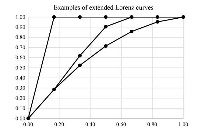
Let X = (x_j) be an (N-1)-sequence of non-negative numbers and let $s_{i}=\sum_{j=1}^{i} x$ be the j^th partial sum. Hence s_N-1 = TOT denotes the total sum of the numbers in X; s₀ is set equal to 0. Now plot the points $\left(\frac{i}{N-1}, \frac{s_{i}}{T O T}\right)_{i=0, \ldots, N-1}$ and connect them by line segments to obtain a curve joining the origin (0,0) with the point (1,1). We refer to this curve as the extended Lorenz curve. Contrary to the standard Lorenz curve this curve is not necessarily concave (but of course still increasing). An example is shown in Figure 3. If X is decreasing then the extended Lorenz curve coincides with the classical Lorenz curve. If X ⋟ Y then the extended Lorenz curve of X is situated above the extended Lorenz curve of Y.

Given the number of nodes, N, we next show a majorization result between the frequency sequence of a complete network K_N, that of a general network G=(V, E), denoted as A, and the frequency sequence C of a chain.

Theorem

Given a network G=(V, E) with N nodes, then,

By (8) and (9) the second inequality means that

And

We moreover prove that

Proof. By (1), we already know that

which proves (11). Assume now that α_i=0, for i > 1, then we already know that ∀ k≥i:α_k=0 and thus

Assume now that for some i > 1, α_i≠0, then we will prove that also in this case $\sum_{j=1}^{i} \alpha_{j} \geq \sum_{j=1}^{i}(N-j)$. This will be done in several steps. First, we show that $\sum_{j=1}^{i} \alpha_{j} \geq \frac{i(i+1)}{2}$. Indeed: there exists in V at least one chain of length i, connecting nodes to which we refer as u₁, u₂, …, u_i+1. Then, by property 6, we know that ∀j=1,…, i: α_j≥i–j+1, and hence $\sum_{j=1}^{i} \alpha_{j} \geq\left(\sum_{j=1}^{i}(i-j+1)\right)=\frac{i(i+1)}{2}$. In the next step, we show that this inequality can be refined to $\sum_{j=1}^{i} \alpha_{j} \geq\left(\frac{i(i+1)}{2}\right)+i$. Indeed, as the network under study is connected, there exists a node in the network, denoted as u_i+2, connected to at least one node of the chain u₁, u₂, …, u_i+1. This point u_i+2 has a distance d, 0 < d ≤ i to at least i points in the chain. Now, adding the i distances involving the point u_i+2 we obtain $\sum_{j=1}^{i} \alpha_{j} \geq\left(\frac{i(i+1)}{2}\right)+i$. We further note that ∀j ≤i, each point in the set S ={u₁, u₂, …, u_i+2} has at least j points in the set S at a distance 0 < d ≤ j.

Now we continue in this way. Assuming that we have a set T of i+n+1 connected nodes {u₁, …, u_i+1, u_i+2, …, u_i+n+1} from which we already derived that $\sum_{j=1}^{i} \alpha_{j} \geq\left(\frac{i(i+1)}{2}\right)+(n i)$ and for which we know that ∀j ≤i each point in the set T, has at least j points in the set T at a distance 0 < d ≤ j. We again apply connectedness to get a new node u_i+n+2 at a distance d, 0 < d ≤ i to all points in T, leading to $\sum_{j=1}^{i} \alpha_{j} \geq\left(\frac{i(i+1)}{2}\right)+(n+1) i$. Again we observe that ∀j ≤i, each point in T* = {u₁, …, u_i+1, u_i+2, …, u_i+n+2} has a distance d, 0 < d ≤ j, with at least j points in the set T*. This procedure ends with n = N-i-2 for which $\sum_{j=1}^{i} \alpha_{j} \geq\left(\frac{i(i+1)}{2}\right)+(N-i-1) i$ =$N i-\sum_{j=1}^{i} j=\sum_{j=1}^{i}(N-j)$ which proves the inequality in the case α_i≠0, and hence (10).

Now we prove (12). Using (10) and (11) we have:

where we still have to prove the final equality in (12). For this, we first observe that:

Now,

1) It follows immediately from the previous theorem that for a given number N and α-array A=(α₁, α₂, …, α_N-1) the median of A is smaller than or equal to the median of the chain of length N-1 (N nodes).

2) It is always possible to find a network with N (N > 3) nodes such that α_i< β_i, and this for each number i=1,…, N-1. Indeed, consider for N > 3, a network for which ∀i, i=1,…,N–3, α_i ≠0; α_N–2=1 and α_N–1=0. In this case α_N–1=0<β_N–1=1; α_N–2=1< β_N–2=3 and, using (12), ∀i, i=1,…, N–3, $\alpha_{i}<\sum_{j=i}^{N-2} \alpha_{j}=\sum_{j=i}^{N-1} \alpha_{j} \leq \beta_{i}$. Such a network may look like shown in Figure 1.

3) The inequality $\alpha_{i} \leq \beta_{i}$ cannot be made more precise as for a chain of length i, α_i=β_i=1, for each i=1,…, N-1.

4) If N > 2, then it is impossible that ∀i=1,…,N–1,α_i=β_iIndeed: $\beta_{1}=\frac{N(N-1)}{2}$ and if α₁ = $\frac{N(N-1)}{2}$ then automatically α_i=0, i=2,.., N–1, while this is not the case for β_i.

5) If A is an array of length N-1, consisting of non-negative natural numbers such that

then the components of A do not have to be frequencies of distances in a network. Indeed, let N = 4 and let A = (4,1,1), then (4,1,1)⋟C=(3,2,1). Yet, there does not exist a network with (4,1,1) as distance frequencies: the third component is equal to one indicating that the network must be a chain but for a chain with 4 nodes, α₁= 3 and not 4.

Even if the last component of A is zero a counterexample is possible. Indeed, with N=5, we have (4,3,3,0) ⋟C=(4,3,2,1). Such a network must have at least one chain of length three (connecting four nodes). The fifth node must be connected to the second or the third node in the chain. Hence A must necessarily be (4,4,2,0) and cannot be (4,3,3,0). These examples lead to the open question of finding the conditions under which such an array A is the frequency array of the distances in a (connected) network.

6) From the above and the main theorem we see that max {Md; Md is the median distance in an N-node network} is strictly smaller than max {$\bar{d}: \bar{d}$ is the average distance of an N-node network}. Although Md ≤ $\bar{d}$ is not always true: a star with a center and N-1 rays (N>4) is an example (Md = 2 and $\bar{d}=\frac{2(N-1)}{N}<2$), we have that if the α – sequence of a network is decreasing then clearly Md ≤ $\bar{d}$. The reverse of this result does not hold in general. This is illustrated by G₀ (N=7) in Figure 2 below. Its α–sequence is not decreasing, namely (6,7,6,2,0,0) but yet Md = 2 < $\bar{d}$ = 46/21 ≈ 2.19.

If N is fixed and the array A=(α₁, α₂,…,α_N–1) denotes the frequencies of the distances in a network, then $\frac{2}{N(N-1)} \sum_{i=1}^{N-1} i \alpha_{i}$ denotes the average distance between nodes in this network, say $\bar{d}$.

Theorem. If $A^{(1)}=\left(\alpha_{1}^{(1)}, \alpha_{2}^{(1)}, \ldots, \alpha_{N-1}^{(1)}\right) \succcurlyeq A^{(2)}=\left(\alpha_{1}^{(2)}, \alpha_{2}^{(2)}, \ldots, \alpha_{N-1}^{(2)}\right)$ then $\overline{d_{1}} \leq \overline{d_{2}}$.

Proof. As $A^{(1)}=\left(\alpha_{1}^{(1)}, \alpha_{2}^{(1)}, \ldots, \alpha_{N-1}^{(1)}\right) \succ A^{(2)}=\left(\alpha_{1}^{(2)}, \alpha_{2}^{(2)}, \ldots, \alpha_{N-1}^{(2)}\right)$, we know that

$\forall i=1, \ldots, N-2: \sum_{j=1}^{i} \alpha_{j}^{(1)} \geq \sum_{j=1}^{i} \alpha_{j}^{(2)} \text { and } \sum_{j=1}^{N-1} \alpha_{j}^{(1)}=\sum_{j=1}^{N-1} \alpha_{j}^{(2)}$. Consequently: ∀i=2,…,N–2:$ \sum_{j=i}^{N-1} \alpha_{j}^{(1)} \leq \sum_{j=i}^{N-1} \alpha_{j}^{(2)}$.

$\begin{array}{l} \text{Now,} \overline{d_{1}}=\frac{2}{N(N-1)} \sum_{j=1}^{N-1} j \alpha_{j}^{(1)} \\ =\frac{2}{N(N-1)}\left[\sum_{j=1}^{N-1} \alpha_{j}^{(1)}+\sum_{j=2}^{N-1} \alpha_{j}^{(1)}+\ldots+\sum_{j=N-1}^{N-1} \alpha_{j}^{(1)}\right] \\ \leq \frac{2}{N(N-1)}\left[\sum_{j=1}^{N-1} \alpha_{j}^{(2)}+\sum_{j=2}^{N-1} \alpha_{j}^{(2)}+\ldots+\sum_{j=N-1}^{N-1} \alpha_{j}^{(2)}\right] \\ =\frac{2}{N(N-1)} \sum_{j=1}^{N-1} j \alpha_{j}^{(2)}=\overline{d_{2}} \end{array}$

Corollary. It follows from the previous theorem that the average distance between nodes in an N-node network is at most equal to the average distance in an N-node chain, namely $\frac{(N+1)}{3}$ (see the appendix for the simple calculation of this value).

Remark. If G(A) denotes the Gini index of the array A of distance frequencies, we have

Hence, the Gini coefficient respects the extended majorization order. From (13) one can express $\bar{d}$ as a function of G(A):

The previous theorem shows that the operation of taking the average distance in an N-node network respects the opposite of the Lorenz majorization order, while the Gini coefficient respects this order.

Assume that we have an N-node chain, hence containing N-1 links. Then its set of distances contains $\frac{(N-1) N}{2}$ numbers and the median, Md, is either a natural number m or m-0.5. Then we have

As for each natural number j, we have $\sum_{k=1}^{N-j} k=\frac{(N-j)(N-j+1)}{2}$, we can prove that m = [x] with

from which it follows that $x=\frac{(2 N+1)-\sqrt{2 N^{2}-2 N+1}}{2}$ and hence Md is either [x]-05 or [x]. For N large this leads to

Consequently, $\lim _{N \rightarrow \infty} \frac{M d}{\bar{d}}=3\left(1-\frac{\sqrt{2}}{2}\right) \approx 0.879<1$.

Moreover, we see that Md < $\bar{d} \Leftrightarrow N+\frac{1}{2}-\frac{\sqrt{2}}{2} \sqrt{N^{2}-N+\frac{1}{2}}<\frac{N+1}{3} \Leftrightarrow$ N²–13N+4>0⇔N>12.7. Hence, in practice: N ≥ 13. Checking this manually for N = 2, …,14 we find that also then Md < $\bar{d}$ except for N = 2, 5, 8, and 11 in which cases Md = $\bar{d}$.

The array of G₀ is (6,7,6,2,0,0). Figure 3 shows its extended Lorenz curve, situated between the extended Lorenz curve of K₇ (the complete network on 7 nodes) and the extended Lorenz curve of the chain of length 6. The average distances are respectively equal to 1, 2.19, and 2.67; the medians are 1, 2, and 2; while the corresponding Gini coefficients are: 0.833, 0.437, and 0.278.

In this article, we introduced the study of the distance distribution of a network. We showed that the distance distribution in an undirected network majorizes the one of a chain and is always smaller (in the sense of majorization) than the distribution of the corresponding complete N-network. The Gini coefficient respects the majorization order for such distributions, while the average distance behaves oppositely. As a consequence, the average and median distances in any such network are smaller than those of a chain.

We intend to use these results in the study of small worlds and the so-called six degrees of separation property (work in preparation).

The author thanks his colleague Ronald Rousseau for useful discussions.

Proof that the average distance in an N-node chain is $\frac{(N+1)}{3}$

The average distance in an N-node chain is equal to