


1 Introduction
Smart communities represent a transformative paradigm in urban development. By integrating advanced technologies, they enhance the functionality, sustainability, and livability of urban built environments (Zaidan et al., 2022). At the heart of this evolution is artificial intelligence (AI), which enables intelligent management of community resources—from energy-efficient buildings to responsive urban infrastructure(Zygiaris, 2013). With over 55 percent of the global population now residing in urban areas—a share projected to rise to 68 percent by 2050—smart communities, as integral components of smart cities, serve as critical testbeds for AI applications (Stratigea, 2012). As urbanization accelerates and residents’ needs become increasingly diverse, the development of smart communities has emerged as a vital strategy for enhancing urban management efficiency and improving quality of life. However, this process also faces several challenges, including technical integration, data security, and financial investment. The rapid advancement of information technology presents new opportunities for developing smart communities (Allam & Dhunny, 2019). However, effectively integrating the Internet of Things (IoT), big data, cloud computing, and artificial intelligence—while ensuring data security and privacy—remains a significant challenge (Belanger et al., 2002; Zhang et al., 2018). Furthermore, the sustainability of smart communities has attracted attention from various fields, including architecture, information technology, and sociology (Bibri & Krogstie, 2017), due to their potential to enhance management efficiency, promote sustainable urban development, and foster social harmony. Bibliometric analysis not only provides a comprehensive review of development trends in the smart-community field but also uncovers the key scholarly actors, patterns of international collaboration, and potential directions for future research. This approach greatly facilitates a systematic investigation of smart communities and offers more strategic guidance for subsequent academic studies and practical applications.
Since the International Telecommunication Union first defined a smart community in 1992 as one that utilizes digital organizational principles, tools, and innovative methods to promote sustainability, inclusiveness, success, and creativity, research on smart communities has steadily deepened and broadened (Goldsmith & Crawford, 2014; Mylonas et al., 2021). In 2011, Li et al. (2011) proposed a multilayered architecture for smart communities, integrating households, communities, and services. This framework laid the foundation for complex Internet of Things (IoT) applications and expanded the concept of smart home. Kim et al. (2014) investigated a smart-community model in residential neighborhoods through a placemaking lens. They employed mobile augmented reality to stimulate resident engagement, but the study’s reliance on a single housing estate limits its broader applicability. In contrast, Bibri and Krogstie (2017) emphasized the evaluation of sustainable smart cities from an interdisciplinary perspective. In 2018, with the emergence of a new energy sector, Su et al. (2018) introduced a blockchain-based secure charging solution that enhanced the applications of smart communities in energy management. In 2020, Woolliscroft (2020) integrated smart communities with healthcare efficiency, advocating for an interdisciplinary approach that fosters collaboration among various stakeholders to improve healthcare services. In 2021, Mylonas et al. (2021) emphasized that the adoption of digital twin technology in smart cities necessitates community engagement, highlighting the significance of collective involvement. In 2022, Ding et al. (2022) explored the role of smart communities in COVID-19 governance, demonstrating their potential in public health and civic participation. Jiang (2022) developed a dynamic, big-data-driven analysis model for smart communities using logistic regression, which demonstrated superior accuracy in forecasting community service demands. Sakshi et al. (2023) employed a hybrid analytical approach to survey core themes and methodological paradigms in smart-community research, mapping global hotspots and their evolutionary trajectories. Rehman et al. (2023) proposed the Selfishness Elimination (SOS) mechanism to improve the collaborative efficiency of Internet of Things (IoT) devices within smart communities. However, they did not validate its scalability under large-scale deployment (Rehman et al., 2023). In 2023, Zuo and Chen (2023) proposed optimizing public services within smart communities using big data, thereby enhancing service efficiency and resource utilization. In 2024, Niu et al. (2024) stressed the importance of bolstering community resilience by increasing the level of intelligence, thereby strengthening the capacity of smart communities to address uncertainty and vulnerability.
To date, research on smart communities has primarily focused on integrating intelligent technologies with social needs, thereby promoting efficient, inclusive, and sustainable community development (Bibri & Krogstie, 2017). Existing studies have predominantly concentrated on single domains, such as energy management, public safety, or health services, without developing solutions that address the diverse needs of communities (including transportation, culture, and education). Few investigations have designed platform functionalities from the perspective of resident experience, and discussions on privacy protection and ethical compliance in big data and AI applications remain limited. Although certain studies offer in-depth analyses of individual technologies or applications, no comprehensive theoretical model currently integrates technological implementation, governance frameworks, service provision, user engagement, and sustainability assessment. Moreover, research on dynamic evolution and emerging trends in this field is lacking. Therefore, this study applies bibliometric analysis to review the development trajectory and present state of smart communities, aiming to provide readers with an intuitive understanding of future research gaps and practical application focal points and to project forthcoming trends. In conducting this research, the study employs bibliometric analysis and utilizes two primary tools, CiteSpace and VOSviewer, to examine relevant publications on smart communities from the Web of Science (WOS) database over the past two decades (2000-2024). This methodology enables us to systematically investigate the current state, focal points, and trends in international smart community research, thereby providing valuable insights and a foundation for future studies and practices. By integrating these tools, this study aimed to address the following research questions (RQs):
RQ1: How have the annual publication volume and disciplinary distribution in the smart-community field evolved between 2000 and 2024?
RQ2: Which journals have a significant impact in the field of smart communities, and how can their research inform future directions?
RQ3: Which countries have played a leading role in smart community research, and what are the characteristics of their collaborative networks?
RQ4: Who are the primary contributing researchers in the field of smart communities, and what challenges or perspectives have they proposed regarding the development of smart communities?
RQ5: Which institutions are the leading contributors to smart community research? What lessons can be learned from their collaborations, and what aspects should be improved in future inter-institutional partnerships?
RQ6: What are the current hotspot themes and emerging directions in smart community research, and how do existing studies align with United Nations Sustainable Development Goal 11 (Sustainable Cities and Communities)?
2 Materials and methods
2.1 Data sources
The data for this study were obtained from the Web of Science (WOS) Core Collection, which comprises three citation index sections: the Science Citation Index Expanded (SCI-Expanded), Social Sciences Citation Index (SSCI), and Arts & Humanities Citation Index (A&HCI). These databases serve as essential sources of high-quality academic literature on a global scale, encompassing core journals in the natural sciences, social sciences, and humanities. They provide a comprehensive and authoritative foundation for conducting bibliometric analyses.
2.2 Search strategy
For the sake of conceptual uniformity, this study defines a “smart community” as a management model supported by information technologies and intelligent systems. Through multi-stakeholder collaborative governance, resource sharing, and application innovation, it seeks to achieve sustainable development across the economic, social, and environmental dimensions of the community (Allam & Dhunny, 2019). In the search strategy, this study incorporated the synonyms smart community, intelligent community, digital community, and smart city community. This inclusive approach ensured comprehensive literature retrieval. The literature search was conducted on December 4, 2024. The search query was set as follows: TS = (“Smart Community” OR “Intelligent Community” OR “Digital Community” OR “Smart City Community”). The search was restricted to the time span of 2000 to 2024, yielding a total of 436 articles. Document types were limited to “Article” and “Review Article,” and the language was limited to English. During the initial screening, 72 articles were excluded for failing to meet the inclusion criteria. The excluded items included News Items lacking original research content (n=1); Corrections issued solely to amend errors (n=1); Meeting Abstracts without complete research data (n=12); Retractions deemed devoid of reference value (n=2); Book Chapters not classified as journal articles (n=2); Editorial Materials offering editors’commentaries rather than novel findings (n=7); Retracted Publications (n=6); Early Access articles that were not formally published and contained incomplete information (n=16); Proceeding Papers subject to inconsistent peer-review standards (n=17); and Non-English publications (n=8). All literature retained for analysis was required to satisfy fundamental scientific criteria, ensuring both comprehensive research content and high publication quality. As a result, 364 articles were retained for further analysis, consisting of 349 research articles and 15 review articles. The detailed screening process is illustrated in Figure 1.
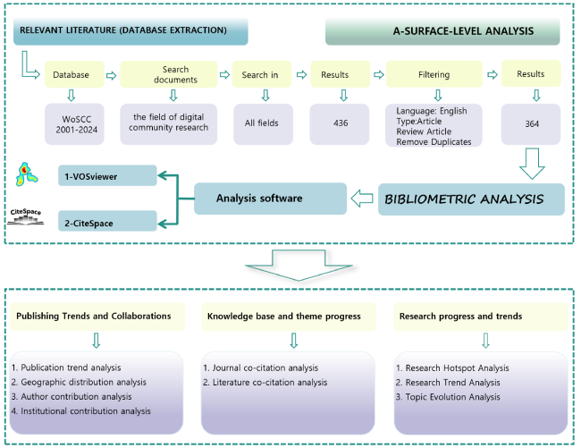
Figure 1. Flowchart of data retrieval and processing. |
2.3 Research methods
Bibliometrics is a quantitative approach rooted in mathematics and statistics, aimed at examining scientific literature along with its production, dissemination, and impact (Bibri & Krogstie, 2017; Glänzel & Moed, 2002). This method unveils a research field’s knowledge structure, hot topics, developmental trends, and scientific communication patterns, constituting a pivotal branch of scientometrics (Kastrin & Hristovski, 2021). Bibliometric analysis provides a structured overview of scientific research by analyzing diverse indicators such as the number of publications, authors, institutions, countries, keywords, journal distributions, and citation relationships. It has broad applications in academic studies, science and technology policymaking, and discipline evaluation (Glänzel & Moed, 2002).
Drawing on publications from 2000 to 2024, this study adopted bibliometric methods to systematically examine research findings from the past 25 years. Preliminary data processing and trend analysis were performed using Microsoft Excel 2021 and annual publication counts were compiled to elucidate the field’s research progress and developmental trends.
To further explore the collaboration networks among countries, authors, and institutions, as well as keyword co-occurrence and emerging themes, this study employed VOSviewer 1.6.20 for network construction and visualization. Developed by Nees Jan van Eck and Ludo Waltman, VOSviewer is designed specifically for handling complex bibliometric networks and boasts powerful visualization capabilities (Van Eck & Waltman, 2010). Additionally, this study leveraged CiteSpace 6.4.R1 for a deeper investigation, including dual-map overlay analyses of journals, co-citation analyses of references, and reference burst detection. CiteSpace, developed by Professor Chaomei Chen’s team, serves as a bibliometric and visualization tool that captures dynamic scientific frontiers and knowledge evolution pathways (Chen, 2003; Wu et al., 2022). CiteSpace is a software tool designed to analyze and visualize the knowledge structure, research hotspots, and developmental trends within scientific literature. VOSviewer excels at constructing and visualizing knowledge networks and maps in this field. By synthesizing these tools, this study offers a multifaceted depiction of the knowledge structure, developmental trajectory, and cooperation patterns in this domain, providing a valuable reference for subsequent research and decision-making.
3 Research results
3.1 Trends in publications and disciplinary distribution
Figure 2 illustrates the annual publication trends in the field of smart community research from 2000 to 2024. Overall, this area of inquiry has experienced a significant upward trajectory. In the early years (2000-2010), the annual publication output was modest, typically remaining in single digits. This limited volume indicates that research on this topic was relatively small in scale at the outset, receiving minimal academic attention. However, as the Internet of Things (IoT), big data, and smart city technologies and concepts gained momentum, researchers’ interest in smart communities gradually increased (Nižetić et al., 2020). From 2013 onward, the volume began to grow rapidly. After 2016, annual publications rose significantly, climbing from just over ten articles per year to more than 20, and surpassing 40 in 2021, an indication of the field’s rapid expansion. Drawing on the exponential fit curve (y=2.7905e0.2063x), which demonstrates a high coefficient of determination (R² = 0.9924), it can be inferred that research in this domain will likely continue growing soon.
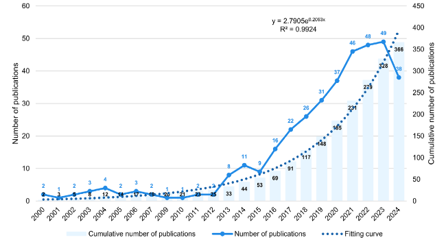
Figure 2. Trend analysis of annual publication volume in smart community research (2000-2024). Notes: The horizontal axis denotes the publication years (2000-2024). The left vertical axis shows the number of publications per year, while the right vertical axis indicates the cumulative total number of publications since 2000. The light blue bars represent the cumulative count of publications for each year, and the solid blue line illustrates the annual publication trend. |
In summary, research on smart communities has progressed from a phase of limited initial exploration to a stage of systematic investigation, reflecting increasing academic attention and investment in the field.
According to the Web of Science classification, 364 articles are distributed across 112 distinct subject categories. Table 1 lists the top 20 categories by publication volume. Engineering, Electrical & Electronic ranks first with 88 articles, followed by Computer Science, Information Systems (62 articles), Telecommunications (62 articles), and Energy & Fuels (59 articles). This pattern reflects the heavy reliance of smart community research on information technology, network communications, and hardware systems and underscores that engineering and computer science serve as its foundational disciplines. This distribution reveals two major trends. First, categories such as Engineering, Electrical & Electronic, and Computer Science, Information Systems have long dominated, indicating that early work focused on underlying networks and hardware architectures. Second, the proportion of publications in environmental and sustainability-oriented fields, most notably Green & Sustainable Science & Technology (21 articles) and Environmental Sciences (18 articles)—has risen steadily. This shift suggests that smart-community research is evolving from a purely technology-driven orientation towards an interdisciplinary integration of ecological and social-governance perspectives.
Table 1. Top 20 disciplines by publication volume. |
| Rank | Web of Science categories | NP | Rank | Web of Science categories | NP |
|---|---|---|---|---|---|
| 1 | Engineering Electrical Electronic | 88 | 11 | Construction Building Technology | 13 |
| 2 | Computer Science Information Systems | 62 | 12 | Computer Science Artificial Intelligence | 12 |
| 3 | Telecommunications | 62 | 13 | Computer Science Interdisciplinary Applications | 11 |
| 4 | Energy Fuels | 59 | 14 | Computer Science Hardware Architecture | 10 |
| 5 | Green Sustainable Science Technology | 21 | 15 | Engineering Civil | 9 |
| 6 | Environmental Sciences | 18 | 16 | Instruments Instrumentation | 9 |
| 7 | Environmental Studies | 16 | 17 | Multidisciplinary Sciences | 9 |
| 8 | Computer Science Theory Methods | 15 | 18 | Public Environmental Occupational Health | 9 |
| 9 | Information Science Library Science | 15 | 19 | Engineering Multidisciplinary | 8 |
| 10 | Communication | 13 | 20 | Social Sciences Interdisciplinary | 8 |
3.2 Knowledge flow analysis
Figure 3 illustrates the multidisciplinary scope of smart community research using the dual-map overlay visualization method proposed by Chen and Leydesdorff (2014). Different journal clusters, corresponding to various academic disciplines, are marked with distinct colors. This visualization, grounded in the global distribution of scientific research, reveals trends in the associated scientific literature (Chen, 2006). The colored curves in the figure represent citation pathways, providing an intuitive view of interdisciplinary connections within smart community research. The left side displays the citing journals, while the right side displays the cited journals. The thickness of the lines indicates the strength of the connections, the thicker the line, the stronger the relationship.
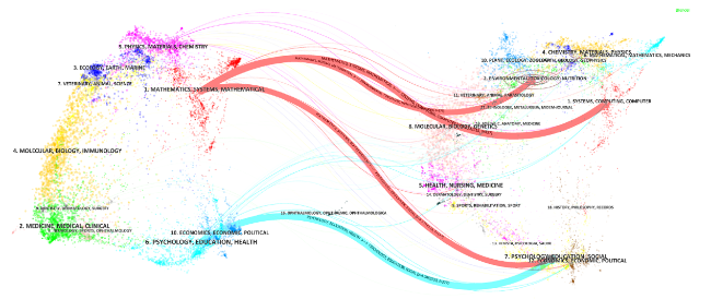
Figure 3. Overlay analysis of two charts for smart community research (2000-2024). Notes: In the overlay map, colors denote the disciplinary categories to which each publication belongs. Lines between nodes indicate citation or referenced-by relationships. Regions composed of densely connected nodes sharing the same color form clusters, each representing a specific academic research domain. |
Figure 3 reveals three principal citation pathways. The first links Mathematics & Systems Science (Cluster 1) to Systems Science, Computational Science & Computer Science (also Cluster 1). The second connects Psychology, Education & Health (Cluster 6) with Psychology, Educational Studies & Social Sciences (Cluster 7). The third runs between Medicine & Clinical Medicine (Cluster 2) and Health, Nursing & Medicine (Cluster 5). These patterns indicate that smart community research is underpinned by mathematical modeling and systems science, with extensive applications in computer science and engineering. At the same time, the field places strong emphasis on both individual mental health and broader public-health concerns, demonstrating an intersection of disciplines such as mathematical systems science, psychosocial health sciences, computer science, and social medicine. The existence of these multiple, multidisciplinary citation linkages underscores the high collaborative potential inherent in smart community research. Because the research questions involve complex systems, human-machine interaction, health management, and community governance, solutions typically require cooperation across diverse fields. The multidisciplinary coupling observed in the citation pathways thus provides empirical evidence of such cross-domain collaboration. This finding further implies that smart community research extends beyond purely technical challenges to encompass broader socio-systemic issues, necessitating sustained, cross-disciplinary partnerships.
3.3 Journal contribution analysis
Table 2 (left panel) lists the top ten journals by publication volume. IEEE Access (United States; IF=3.4) and Energies (Switzerland; IF=3.0) each published 17 articles, making them the most prolific outlets. They are followed by Sustainability (Switzerland; IF=3.3) with 10 articles. These figures indicate that these journals receive extensive attention in smart community research and play a pivotal role in advancing the field. Among these ten journals, Sustainable Cities and Society (Netherlands, IF=10.5) has the highest impact factor. Although it published only four articles, it ranks seventh in total citations (120), reflecting its high-quality influence on sustainability studies within the smart-community domain.
Table 2. Top 10 journals by publication volume and citation frequency. |
| Rank | Journals | NP | Country | IF (JCR2023) | Cited journals or meetings | NC | Country | IF (JCR2023) |
|---|---|---|---|---|---|---|---|---|
| 1 | IEEE ACCESS | 17 | USA | 3.4 | IEEE T SMART GRID | 355 | USA | 8.6 |
| 2 | ENERGIES | 17 | Switzerland | 3.0 | APPL ENERG | 320 | United Kingdom | 10.1 |
| 3 | SUSTAINABILITY | 10 | Switzerland | 3.3 | IEEE ACCESS | 195 | USA | 3.4 |
| 4 | SENSORS | 6 | Switzerland | 3.4 | ENERGY | 184 | United Kingdom | 9.0 |
| 5 | IEEE COMMUNICATIONS MAGAZINE | 5 | USA | 8.3 | RENEW SUST ENERG REV | 164 | USA | 16.3 |
| 6 | APPLIED ENERGY | 5 | United Kingdom | 10.1 | ENERGIES | 164 | Switzerland | 3.0 |
| 7 | ENERGY | 5 | United Kingdom | 9.0 | SUSTAIN CITIES SOC | 120 | Netherlands | 10.5 |
| 8 | PLOS ONE | 5 | USA | 2.9 | IEEE T POWER SYST | 112 | USA | 6.5 |
| 9 | IEEE INTERNET OF THINGS JOURNAL | 4 | USA | 8.2 | IEEE T IND INFORM | 110 | USA | 11.7 |
| 10 | SUSTAINABLE CITIES AND SOCIETY | 4 | Netherlands | 10.5 | SUSTAINABILITY-BASEL | 102 | Switzerland | 3.3 |
Table 2 (right panel) presents the top ten journals by citation frequency. IEEE Transactions on Smart Grid leads with 355 citations. Applied Energy follows with 320 citations, and IEEE Access with 195. This citation profile highlights the strong scholarly recognition of energy and smart grid research in the context of smart communities. It also underscores the significant influence these journals exert on disseminating knowledge and shaping the field’s development.
3.4 National collaboration analysis
The analysis of collaboration among countries and regions reveals the patterns and intensities of scientific partnerships, reflecting the research capabilities and international influence of various nations (Hoekman et al., 2010; Luukkonen et al., 1993). In the field of smart community research, 59 countries have contributed to academic outputs. Table 3 lists the top ten countries by publication volume. China ranks first with an overwhelming lead, contributing 137 publications (NP), more than twice that of the second-ranked United States. This underscores China’s remarkable research activity in this field. Additionally, China’s total citations (NC) reach 2,979, with an average citation per paper (AC) of 21.74 and an H-index of 26. These metrics indicate that Chinese academic research demonstrates both quality and influence.
Table 3. Top 10 countries by publication volume. |
| Rank | Country | NP | NC | AC | H-index |
|---|---|---|---|---|---|
| 1 | China | 137 | 2,979 | 21.74 | 26 |
| 2 | USA | 68 | 1,570 | 23.09 | 20 |
| 3 | Japan | 30 | 331 | 11.03 | 9 |
| 4 | Canada | 23 | 767 | 33.35 | 11 |
| 5 | Italy | 23 | 621 | 27.00 | 11 |
| 6 | Australia | 22 | 1,164 | 52.91 | 12 |
| 7 | Pakistan | 21 | 561 | 26.71 | 12 |
| 8 | United Kingdom | 21 | 313 | 14.90 | 10 |
| 9 | Spain | 20 | 396 | 19.80 | 10 |
| 10 | Saudi Arabia | 20 | 378 | 18.90 | 10 |
The United States ranks second with 68 publications, 1,570 total citations, and a higher average citation per paper (AC) of 23.09 compared to China. This suggests that while the U.S. has fewer publications, its research outputs exhibit stronger academic quality and citation impact. Among European countries, Italy and Spain display similar academic performance, with 23 and 20 publications, respectively. Their total citations are 621 and 396, resulting in average citation counts of 27.00 and 19.80, respectively, highlighting stable and high-quality academic contributions.
China (137 publications) and the United States (68 publications) consistently rank first in smart community research output, reflecting their leading positions driven by supportive policies and substantial funding. Canada, although responsible for only 23 publications, commands the highest academic attention with an average citation rate of 33.35, evidencing its outstanding research quality. Emerging contributors, such as Australia (22 publications, average citations=52.91) and Pakistan (21 publications, average citations=26.71), have also shown strong performance; notably, Australia’s field-weighted citation impact exceeds 1.2, underscoring its innovative potential in sustainable and intelligent energy research. Regionally, Asia and North America form dual research hubs, followed by Europe. To promote the global exchange and integration of smart-community technologies and governance strategies, it is advisable to strengthen intercontinental collaboration.
As shown in Figure 4, a visual analysis of collaboration relationships between countries was conducted using VOSviewer software. The minimum publication threshold for countries was set at 5 articles. The resulting network map of country collaborations reveals the distribution and intensity of cooperation among nations. In the map, the size of the circles represents the publication volume of each country, with larger circles indicating higher publication volumes. The thickness of the connecting lines reflects the strength of collaboration between countries, with thicker lines indicating stronger cooperation. The gradient color of the lines illustrates the overall intensity of a country’s collaboration with others (Xie et al., 2020).
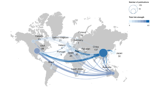
Figure 4. The country collaboration map for smart community research (2000-2024). Notes: The size of the notes indicates the number of publications, while color intensity reflects the strength of collaboration. Edges denote cooperative relationships, with thicker lines signifying closer partnerships. |
From the map, it is evident that China, with 137 publications and a significant level of international cooperation, occupies a central position. China has particularly strong collaborations with several countries, such as the United States, Australia, and the United Kingdom, with thicker lines connecting China to these nations. This indicates that China not only excels in domestic research but also plays a key role in international collaborations. This highlights China’s prominent position in global knowledge exchange and research contributions in this field. The United States, as another major node, has established deep collaboration with several countries, including Canada, Italy, and Australia. Australia, recognized as a leading research force in the Southern Hemisphere, has developed a network of international collaborations mainly concentrated in the Northern Hemisphere, especially with China and the United States.
Overall, international collaboration has played a crucial role in advancing the globalization of smart community research (Komninos, 2009; Schaffers et al., 2011). The collaboration patterns in this field are notable, including high-intensity cooperation among major countries and a certain degree of regional networking. This collaborative model provides a solid foundation for further development in smart community research.
Beyond traditional indicators, this study adopts the Field-Weighted Citation Impact (FWCI) to compare research influence across countries. The FWCI measures the citation performance of an article, journal, or institution relative to global norms within its field (Purkayastha et al., 2019). The average citation for literature in the field of smart design research globally is 18.9, and FWCI = country (AC) / global (AC). China’s FWCI stands at 1.15, slightly above the global average of 1.00, reflecting benefits from the 2012 national smart-city pilot program and the subsequent New-Type Smart City construction plan. The United States achieves an FWCI of 1.22, maintaining its lead through initiatives such as the 2016 Smart City Challenge and substantial federal investment in AI/IoT R&D. Japan records an FWCI of 0.58, marginally below the average. Although its Society 5.0 strategy (launched in 2016) has accelerated smart-community technology development, its academic impact would benefit from broader international collaboration. Canada’s FWCI is 1.76, a result of joining the Global City Teams Challenge in 2017 and launching its own Smart Cities Challenge, which has produced high-quality, policy-oriented research outputs. Australia exhibits the highest FWCI at 2.79, owing to the 2017 National Smart Cities Plan and targeted funding for sustainable energy networks; these measures have driven several highly cited studies on energy management and community optimization. Italy’s FWCI of 1.42 reflects support from its Digital Agenda 2020, which explicitly funds smart community pilots and provides stable financing to domestic universities and research institutes. Spain’s FWCI of 1.04 benefits from the Smart City Expo World Congress, co-organized by government and industry, which facilitates international scholarly exchange in urban management and social governance. These normalized citation metrics, when viewed alongside their respective policy contexts, not only explain the leadership of China and the United States but also highlight the diverse drivers and collaborative synergies underpinning smart community research in other key countries.
3.5 Analysis of author contributions
The analysis of author contributions reveals the collaborative relationships among scholars and their academic networks, aiding in the core researchers who play a leading role in specific research areas (Bozeman et al., 2013; Moody, 2004). In this study, a total of 1,417 authors have contributed. Table 4 lists the top ten authors ranked by publication volume.
Table 4. Top 10 authors by publication volume. |
| Rank | Author | NP | NC | AC | H-index |
|---|---|---|---|---|---|
| 1 | Gao, Weijun | 8 | 179 | 22.38 | 5 |
| 2 | Javaid, Nadeem | 7 | 132 | 18.86 | 7 |
| 3 | Qian, Fanyue | 6 | 138 | 23.00 | 3 |
| 4 | Gu, Tiantian | 5 | 25 | 5.00 | 2 |
| 5 | Aurangzeb, Khursheed | 4 | 92 | 23.00 | 3 |
| 6 | Liu, Yang | 4 | 61 | 15.25 | 3 |
| 7 | Romero-Cadaval, Enrique | 4 | 56 | 14.00 | 4 |
| 8 | Wang, Chenyang | 4 | 23 | 5.75 | 2 |
| 9 | Hao, Enyang | 4 | 17 | 4.25 | 2 |
| 10 | Smith, David B. | 3 | 391 | 130.33 | 3 |
Gao Weijun leads in productivity with eight published papers, though his average citation count (AC=22.38) is slightly lower than Qian Fanyue’s (AC=23.00). In contrast, David B. Smith, with only three publications, attains an exceptional average citation rate (AC=130.33), demonstrating the outstanding scholarly quality of his work. Javaid Nadeem and Aurangzeb Khursheed both maintain h-indices of seven or above, reflecting efficient team collaboration and sustained academic output. Meanwhile, mid-level contributors, such as Gu Tiantian and Hao Enyang, have rapidly attracted attention by concentrating on cutting-edge topics, such as blockchain and digital twins. Overall, these patterns indicate that future author-team development should balance publication volume with scholarly impact. We therefore recommend drawing on the success of a small number of high-impact studies and fostering cross-team collaboration to drive innovative research.
This study used VOSviewer software to visualize collaboration relationships among authors. By setting the minimum publication threshold to three papers, a collaboration network involving 24 authors was generated (Figure 5). In the figure, nodes represent authors, with the size of each node proportional to the number of publications, and the lines between nodes represent collaborative relationships among the authors (Qiu et al., 2014).
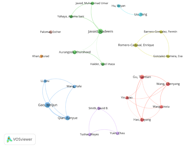
Figure 5. Author collaboration network in smart community research (2000-2024). Notes: Each node represents a single author, with the node size proportional to the author’s publication count. Edges denote co-authorship relationships. Clusters of similarly colored nodes indicate distinct collaboration groups. The spatial proximity of any two nodes reflects the frequency of their collaboration—nodes positioned closer together have collaborated more often. |
As shown in Figure 4, the green node cluster centered around Javaid Nadeem is particularly prominent, indicating its core position within the collaboration network. The network led by Javaid Nadeem includes several scholars, such as Yahaya Adamu Sani, Aurangzeb Khursheed, and Syed Irtaza, highlighting his role as a key cooperation hub. This collaboration model, with core authors at its center, reflects Javaid Nadeem’s significant academic influence in the field of smart community research. Additionally, the red node cluster centered around Gu Tiantian demonstrates strong collaboration among multiple researchers, including Wang Chenyang, Hao Enyang, and Yin Jiyao. This indicates a high frequency of academic exchange and collaboration within this group.
Also noteworthy is the collaboration network centered around Gao Weijun, which is relatively centralized and involves authors such as Li You and Qian Fanyue. This reflects a high level of stability and concentration within the team. Overall, an author’s collaboration network presents a relatively decentralized, yet stable structure, illustrating a diverse collaboration model in academic research (DeLeon & Varda, 2009; Powell et al., 2005).
3.6 Analysis of institutional contributions
Institutional analysis can reveal the overall landscape and key players within a research field, offering valuable insights into the academic influence and collaboration networks of important research institutions (Hollingsworth, 2000). In the field of smart community research, a total of 679 institutions have participated in related studies. Table 5 lists the top ten institutions based on publication volume, visually presenting the distribution of research in this field and the academic impact of each institution.
Table 5. Top 10 institutions by publication volume. |
| Rank | Organization | NP | NC | AC | H-index |
|---|---|---|---|---|---|
| 1 | KING SAUD UNIV | 13 | 314 | 24.15 | 9 |
| 2 | TONGJI UNIV | 9 | 213 | 23.67 | 5 |
| 3 | COMSATS UNIV ISLAMABAD | 8 | 238 | 29.75 | 7 |
| 4 | UNIV KITAKYUSHU | 8 | 179 | 22.38 | 5 |
| 5 | CHINA UNIV MIN & TECHNOL | 7 | 73 | 10.43 | 4 |
| 6 | NORTH CHINA ELECT POWER UNIV | 6 | 132 | 22.00 | 5 |
| 7 | QINGDAO UNIV TECHNOL | 6 | 114 | 19.00 | 3 |
| 8 | SICHUAN UNIV | 6 | 83 | 13.83 | 5 |
| 9 | ZHEJIANG UNIV | 5 | 791 | 158.20 | 5 |
| 10 | CHINESE ACAD SCI | 5 | 133 | 26.60 | 3 |
King Saud University leads the field with 13 published papers, demonstrating outstanding research performance. It has accumulated 314 total citations (NC), an average of 24.15 citations per paper (AC), and an H-index of 9, underscoring its significant academic influence in smart-community research. Tongji University follows with nine publications, 213 total citations (AC=23.67), and an H-index of 5, reflecting its substantial contributions to both quantity and quality.
COMSATS University Islamabad and the University of Kitakyushu have each produced eight papers. COMSATS’s average citation rate of 29.75 highlights the broad impact of its output, while the University of Kitakyushu’s AC of 22.38 also attests to its strong scholarly standing. Particularly noteworthy is Zhejiang University: despite only five publications, it has garnered 791 citations in total, averaging 158.20 citations per paper, which signals exceptional research quality and international reach.
Regionally, institutions in the Middle East, China, and Pakistan each exhibit unique strengths, illustrating a trend towards internationally coordinated, multi-center research. Emerging entities, such as COMSATS University Islamabad and North China Electric Power University, further demonstrate significant academic potential.
Overall, the high output and citation impact of these core institutions not only shape the smart community research landscape but also provide crucial benchmarks for future collaboration and scholarly exchange. To further promote cross-regional knowledge sharing and technology transfer, it is recommended to strengthen joint research initiatives among high-impact institutions that presently engage in relatively limited cooperation.
This study utilized VOSviewer software to visually analyze collaborative relationships among institutions. By setting a minimum publication threshold of three papers, a cooperation network map was generated, comprising 35 institutions (see Figure 6). In the map, nodes represent the institutions, and the lines between nodes indicate collaborative relationships.
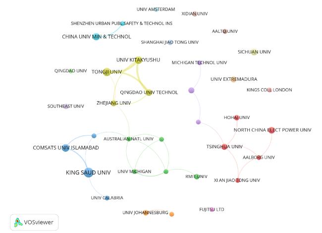
Figure 6. Institutional collaboration network in smart community research (2000-2024). Notes: Each node represents a distinct institution, with node size proportional to its total number of publications. Edges between nodes indicate collaborative relationships, and their thickness corresponds to collaboration strength. Node colors distinguish different collaboration clusters, and the spatial proximity of any two nodes reflects the frequency of their cooperation—nodes positioned closer. |
The analysis reveals that King Saud University occupies a central position within the network, forming close collaborations with several international universities and research institutions, including COMSATS University Islamabad, the University of Michigan, and the University of Calabria. The broadness of this collaboration network highlights its dominant role in the research field. Chinese institutions form a distinct regional cluster within the cooperation network. Centered around Tongji University, there is particularly close cooperation with Zhejiang University, Qingdao University of Technology, and China University of Mining and Technology. This regional collaboration pattern reflects the frequent interactions and collaboration of Chinese universities in the field of smart community research, showcasing the collective advantages and synergistic effects of domestic academic research.
Additionally, there are some relatively isolated institutions within the network, such as Fujitsu Ltd., Sichuan University, and Aalto University. In the future, these institutions are expected to enhance their academic output and increase their influence in the field by strengthening inter-institutional cooperation, particularly with the core network. This collaboration network reveals the patterns of cooperation among institutions engaged in the field of smart community research and highlights the characteristics of international and regional collaborations, providing a valuable reference for future cross-institutional research.
3.7 Research knowledge bases
Bibliometric co-citation analysis is an important method for scholars to uncover potential connections, research hotspots, and development trends within a knowledge field (Hou et al., 2018). When both Document A and Document B are cited by the same Document C, a co-citation relationship is established between A and B (Boyack & Klavans, 2010). This study employed the g-index (k=25) to extract and identify 605 references from the 364 articles included, followed by co-citation and clustering analysis of these references. The aim of this process is to explore the core knowledge structure of the field and trace the evolution of its key themes (Liu et al., 2015).
Figure 7 displays the co-citation network of references, highlighting 14 highly cited articles, with labels indicating the first author and publication year. In the network, the most frequently cited article is authored by Qi and Guo, published in 2019 in the International Journal of Distributed Sensor Networks, titled “Development of a Smart City Community Service Integrated Management Platform” (Qi & Guo, 2019). This article has been cited six times, demonstrating its significant influence in the research field. This study focuses on the development of an integrated management platform for smart city community services, aiming to address inefficiencies and unequal resource distribution in traditional community services. By integrating IoT, big data, and cloud computing technologies, the platform enables intelligent and unified management of community services.
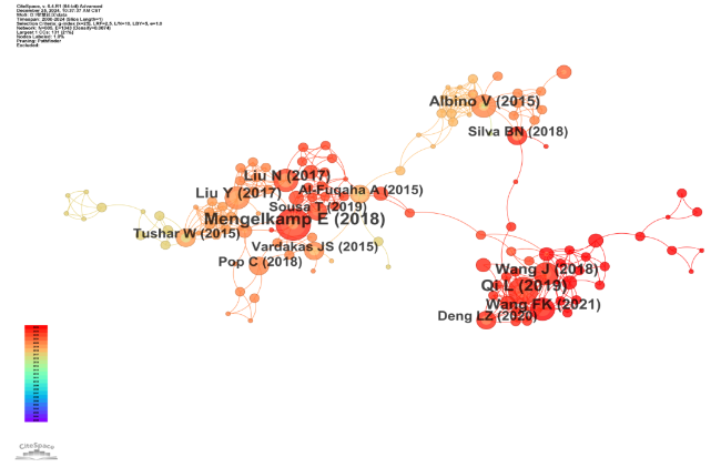
Figure 7. Co-citation network of references in smart community research (2000-2024). Notes: In this visualization, each node corresponds to a single publication, with the node size proportional to its co-citation frequency. The edges between nodes indicate co-citation links. Node colors are assigned by a time-heat algorithm to reflect different temporal co-citation periods: red hues denote recent high-frequency co-citations, while blue-green hues indicate earlier citation hotspots. |
As shown in Figure 8, building on this, we conducted a clustering network analysis of the references. Using the Log-Likelihood Ratio (LLR) algorithm, clustering labels were extracted from the article titles, and four major clusters were identified from the 605 references. The clustering analysis results show that the Q value is 0.9472 (greater than 0.3), indicating a significant clustering structure, and the S value is 0.9582 (greater than 0.7), suggesting that the clustering results are highly reliable. As shown in Figure 8, the clustering network divides the following four major themes: #0 Techno-economic performance, #1 Smart community construction, #2 Intertwining development driver, and #3 Electric vehicle. First, Cluster #0 Techno-economic Performance focuses on the cost-benefit analysis and life-cycle assessment of IoT and intelligent sensing systems. Manfren et al. (2021) demonstrate that by optimizing device selection, energy-efficiency cost savings of 10%-25% can be achieved. Second, Cluster #1 Smart Community Construction emphasizes platform-based governance and resident participation; Li and Zhang (2024) used a qualitative comparative analysis (QCA) of 52 pilot regions, identified community governance, public-private partnerships (PPP), and intelligent service platforms as its core elements. Third, Cluster #2 Intertwining Development Drivers explores the synergistic effects of policy guidance, financial incentives, and social capital. Bokolo (2023) proposed that community engagement is the key driver of co-innovative governance and constructed a multi-stakeholder co-governance model. Finally, Cluster #3 Electric Vehicles regards EVs as mobile storage units within smart communities, with V2G technology showing promise for demand response and microgrid resilience. Xue et al. (2021) verified, within a coupled transportation-electricity framework, that system reliability is optimal when the EV-to-DG capacity ratio is 3:1.
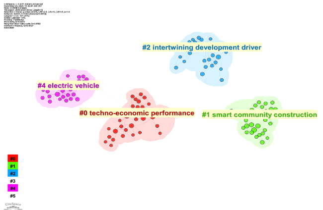
Figure 8. Reference clustering map for smart community research (2000-2024). Notes: In this visualization, each node represents a cited reference, and edges between nodes indicate co-citation relationships. Distinct colors delineate multiple clusters, each corresponding to a specific knowledge subfield. Every cluster is labeled with high-frequency terms automatically extracted by the system, and cluster identifiers begin at #0, with smaller numbers denoting larger cluster size and greater centrality. |
The burst detection analysis reflects the rapid growth of research hotspots over a specific period. The higher the burst intensity, the greater the influence of the document during that timeframe (Jin et al., 2017; Zhou et al., 2019). Figure 9 presents the top 13 references with the most significant burst intensities from 2000 to 2024. Among them, the article by Qi and Guo (2019) has the highest burst intensity of 3.07, making it the most influential paper in recent years regarding smart community research. This study focuses on the application of distributed sensor networks in smart communities, particularly highlighting their crucial role in data collection and processing. The second-ranked article is by Li et al. (2011), with a burst intensity of 3.00. This study explores the overall framework design of smart cities (with smart communities as a key subfield) from the perspective of communication technology, with particular emphasis on the integration of the Internet of Things (IoT) and next-generation networks (5G). Ranked third is the article by Liu and Hu (2016), with a burst intensity of 2.73. This study delves into resource scheduling and optimization issues in large-scale distributed computing within smart communities, proposing an innovative dynamic resource allocation algorithm that significantly enhances computational efficiency and system stability in a complex smart community environment (Liu & Hu, 2016).
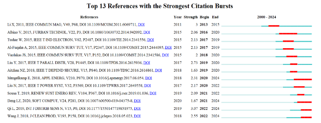
Figure 9. Citation-burst timeline of references in smart community research (2000-2024). Notes: The horizontal axis denotes years; the red bars indicate the periods during which a reference experienced a citation burst. Each row corresponds to a reference with high burst strength, where “burst strength” quantifies the rapid increase in citation frequency over a short interval. The begin-end years specify the exact period of each citation burst. |
3.8 Co-occurrence evolution
Co-occurrence analysis examines frequently occurring keywords and terms in the literature to uncover the relationships between them (Radhakrishnan et al., 2017). This method aims to illustrate the thematic structure of the literature, establish connections between studies, trace historical research hotspots, and speculate on potential future development directions. By analyzing keyword co-occurrence, this approach helps identify prominent themes and emerging trends within a research field, providing valuable insights into the evolution of scholarly discourse and guiding future research inquiries (Liu et al., 2022).
3.8.1 Keyword co-occurrence analysis
This study employed VOSviewer to conduct keyword co-occurrence analysis. Keywords were grouped into clusters based on their co-occurrence frequencies and intrinsic relationships, thereby highlighting research hotspots and thematic evolution within the smart community domain. The co-occurrence network was built using a combination of author keywords and title keywords, with co-occurrence frequency as the similarity measure. To balance network coverage against noise, the minimum co-occurrence threshold was set to three, which excluded low-frequency terms with limited informational value and enhanced the stability and interpretability of the cluster solutions (Bao et al., 2025). Clustering was performed using VOSviewer’s default VOS clustering algorithm, which partitioned the network into five clusters, each shown in a different color (Figure 10A). The density visualization (Figure 10B) then maps the heat distribution of keywords, further highlighting the regions of concentrated research activity.
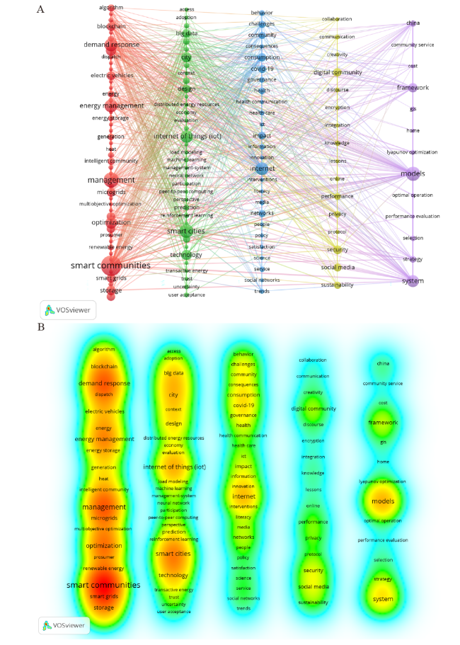
Figure 10. Keyword clustering diagram: (A) Keyword co-occurrence, (B) Keyword density. Notes: In Figure 10A, each node represents a high-frequency keyword, and edges indicate instances of two keywords co-occurring in the same document. The node colors correspond to clusters automatically detected by VOSviewer, the node size reflects the frequency of each keyword, and the density of connecting lines denotes the strength of co-occurrence with other keywords. In Figure 10B, the color gradient encodes co-occurrence frequency: cooler tones (blue) indicate lower frequencies, while warmer tones (red) signify higher frequencies. |
Cluster #1: This cluster revolves around core issues related to smart communities in the fields of energy management, emphasizing the heightened focus on energy utilization and scheduling. The primary keywords in this cluster include energy management, demand response, renewable energy, microgrids, blockchain, and prosumer, reflecting the researchers’ dual focus on optimizing the balance between energy supply and demand at the community level, while also addressing the multifaceted goals of economic, social, and environmental benefits(O’Dwyer et al., 2019). With technologies such as microgrids and blockchains, the prosumer model enables two-way interactions between community residents and energy providers. This not only meets individual energy independence needs but also enhances the overall energy efficiency and sustainability of the community.
Cluster #2:The text underscores the pivotal role of data and technology in the development of smart communities, highlighting key concepts such as big data, internet of things (IoT), machine learning, neural network, prediction, and reinforcement learning. It emphasizes the importance of leveraging advanced data technologies to derive insights and inform decision-making within smart community research (Sun et al., 2016). By collecting and analyzing multidimensional data on residents’ behaviors and community environments, smart communities can achieve real-time predictions and make optimal decisions in areas such as transportation, energy consumption, and community services. This approach further propels the transformation of urban governance towards enhanced intelligence, precision, and efficiency.
Cluster #3 emphasizes the humanistic and social dimensions of smart communities. Key terms, such as community, behavior, consumption, governance, healthcare, and policy underscore the investigation of smart community development and practices through the lenses of social governance and human-centered care (Malek et al., 2021). This is particularly evident in areas such as public health governance and emergency response, especially during pandemics, where smart communities utilize collaborative mechanisms grounded in social networks and information platforms to swiftly integrate resources and information. This approach facilitates effective cross-departmental and multi-stakeholder coordination. As a result, policymaking and implementation at the community level have consistently evolved, highlighting the significance of the synergistic development of people, technology, institutions, and culture (Berkes, 2009; Healey, 2020).
Cluster #4 focuses on the themes of network and information security, digital applications, and sustainable development. Keywords such as digital community, social media, privacy, security, encryption, and sustainability underscore the significance of digital applications and security governance as fundamental issues within smart communities. Considering the rapid advancements in digital platforms and social media, the challenge of balancing data circulation with user privacy has emerged as a pressing concern for both academia and industry (Dwivedi et al., 2021; Tene & Polonetsky, 2013). Concurrently, the emphasis on sustainability underscores a dual commitment to digitalization and environmental responsibility, promoting community lifestyles that are both eco-friendly and energy-efficient while providing convenient information services. This approach aspires to achieve enduring social and environmental benefits.
Cluster #5 emphasizes macro frameworks, system models, and strategy optimization. Key terms, such as framework, system, models, optimal operation, performance evaluation, strategy, and selection, highlight the significance of systematic planning and holistic management. This perspective offers a structured approach to guide smart communities from high-level planning to practical implementation. Additionally, it underscores the necessity for multi-objective optimization and long-term adaptive evaluation, ensuring that smart community initiatives maintain their effectiveness and resilience over time.
Inter-Cluster Relationships, Governance and IoT occupy central positions in Cluster #3 (Social Governance) and Cluster #2 (Technology-Driven), respectively. These two domains are bridged by the Model node in Cluster #5, indicating that governance models have become the critical hub through which governments, operators, and platform developers orchestrate resources and data in smart-community contexts. Meanwhile, Digital Community (Cluster #4) and Sustainability (present in both Cluster #1 and Cluster #4) co-occur frequently. This pattern suggests that digital services and environmental optimization are no longer pursued in isolation; instead, they advance in parallel via integrated security measures and green technologies, providing residents with both convenience and healthy living conditions.
Cross-Cluster Overlaps, Blockchain appears prominently in both Cluster #1 (Energy Management) and Cluster #4 (Information Security), underscoring its dual role: enabling transaction settlement and microgrid energy-flow tracking, as well as supporting data encryption and privacy protection. Similarly, Deep Learning is the core theme in Cluster #2 (Big Data & Prediction) and a secondary topic in Cluster #5 (System Models), reflecting that algorithmic research simultaneously targets specific applications and overarching framework enhancements.
Evolution of Clusters. In early research, technical themes (Cluster #2) and governance themes (Cluster #3) were largely isolated, indicating a focus on single-dimensional technical tests or policy explorations. As the field matured, Cluster #5 (Models & Frameworks) emerged as a convergence hub, fostering crosspollination among governance, energy management, and security. Recent trends show growing intersections between sustainability and social governance (Cluster #1 ↔ Cluster #3), as well as between deep learning and model optimization (Cluster #2 ↔ Cluster #5). This evolution signals a shift towards deeper interdisciplinary collaboration in smart-community research.
Summary: Cluster analysis reveals that core research scenarios in smart-community studies—from energy scheduling and data privacy to social services—are coordinated around system models. Front-line technologies such as blockchain and deep learning permeate multiple clusters, highlighting the integrated framework of smart communities as a holistic solution that combines technological platforms, governance engines, and sustainable ecosystems. These insights point the way for future cross-domain, cross-sector integrated research.
3.8.2 Hotspot evolution analysis
Figure 11 builds upon the keyword clustering analysis presented in Figure 10, further illustrating the weighted publication years of the keywords. The color gradient, ranging from deep blue to bright yellow, signifies the activity levels of the research topics across various periods. Deep blue denotes early research hotspots, whereas bright yellow indicates recent research trends.
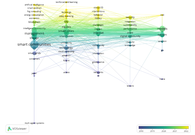
Figure 11. In the keyword time-evolution map for smart community research (2000-2024). Notes: Each node represents a distinct keyword, with node size proportional to its frequency of occurrence. Edges between nodes indicate instances of co-occurrence within the same documents. The node color reflects the period during which the keyword was most active: blue for the early stage, green for the middle stage, and yellow for the recent stage. |
1) Early research concentrated on establishing the technological foundations and intelligent frameworks essential for smart communities, with a focus on keywords such as cloud computing, blockchain, and smart grids. This research primarily addressed the underlying technological infrastructure and application of intelligent systems within these communities (Schaffers et al., 2012). Notably, the potential of blockchain technology for enhancing data security and enabling distributed storage, along with the role of cloud computing in information processing and community services, was emphasized. These technologies provide both theoretical and technical groundwork for subsequent in-depth studies on smart communities.
2) Between 2019 and 2020, the research focus shifted towards the practical application and functional expansion of smart communities. The notable increase in the frequency of keywords such as smart cities, smart homes, and storage technologies suggests that smart communities began to progressively integrate intelligent functions at both urban and household levels (Cvar et al., 2020). Furthermore, research related to technology adoption indicates that scholars are increasingly concentrating on the acceptance and usage rates of smart community technologies within society.
3) Following the years 2021-2022, there has been a notable shift in research trends towards examining the social and environmental impacts of smart communities. The recurrent use of keywords such as sustainability and digital community suggests that scholars have begun to investigate the role of smart communities in promoting sustainable development and fostering community culture. Furthermore, studies addressing COVID-19 have highlighted the significant influence of the global public health crisis on the evolution of smart communities.
4) Recent research trends suggest that smart communities are progressing towards interdisciplinary integration and comprehensive systems. Terms such as models, system integration, and performance evaluation highlight the increasing focus among researchers on the systematic optimization of smart communities. Concurrently, the continuous advancement of technologies like artificial intelligence, reinforcement learning and deep learning is facilitating the intelligent enhancement of these communities.
4 Discussion
4.1 Knowledge framework
In the field of smart community research, existing bibliometric frameworks have predominantly focused on the output analysis and visualization of collaboration networks. Such approaches often overlook in-depth explorations of the intrinsic relationships between core themes and the challenges that lie ahead. For example, Mora et al. (2017) applied co-citation network analysis and development-path identification to smart city literature spanning 1992-2012. Their work revealed two distinct technological trajectories—one led by European academia and the other by the U.S. industry—but did not probe the policy-practice interactions underpinning emerging hotspots. Similarly, Guo et al. (2019) employed VOSviewer and CiteSpace to examine publication outputs, author and institutional collaborations, and keyword bursts in smart city studies from 1998 to 2019. Although their analysis effectively mapped “who publishes” and “what is published,” it fell short of uncovering the deeper connections between research themes or forecasting future challenges. In contrast, the knowledge framework proposed here (Figure 12) moves beyond mere thematic clustering to offer a structured, pillar-based discussion of three core areas: energy management, social governance, and technological integration. For each pillar, the framework systematically delineates both challenges and opportunities. Crucially, it introduces a “challenge-opportunity matrix” that enables readers to visualize research gaps and potential application points briefly. Under the energy management pillar, for instance, the framework not only identifies current technological bottlenecks, but also examines their alignment with the Sustainable Development Goals (SDGs). This dual analysis yields concrete policy recommendations and technical roadmaps for future investigations. Moreover, by mapping each core theme onto the relevant SDGs and integrating policy guidance with technology planning, the framework enhances the practical utility and operational clarity of bibliometric studies. By combining quantitative cluster analysis with qualitative, in-depth discussion, the proposed framework bridges the divide between academic research and real-world practice. This innovative approach not only transcends the limitations of traditional bibliometric methods but also offers more targeted directions for the future development of smart communities.
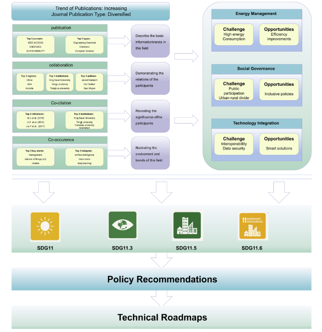
Figure 12. Knowledge framework. |
Through the analysis of publications, it is evident that research in this field continues to hold significant value for further study and practical application. The distribution of publications on smart community research exhibits interdisciplinary characteristics and a strong reliance on information technology. From 2000 to 2024, the volume of publications in this field has steadily increased, with a continuing trend of expansion, indicating promising prospects for research in this area. Specifically, the top three journals with the highest publication volumes are IEEE ACCESS, ENERGIES, and SUSTAINABILITY. In terms of citation frequency, IEEE TRANSACTIONS ON SMART GRID leads, with 355 citations. The core research on smart communities is centered on areas such as multi-energy coordination and optimization, big data analysis, demand-side management, sustainability and resilience, and cybersecurity and privacy protection. Emphasis is placed on implementing these studies in practical community pilot projects and further promoting the large-scale development of smart communities through standardization and policy support.
Collaboration analysis reveals dynamic relationships among countries, institutions, and authors (Abbasi et al., 2011), highlighting key collaborative participants in the field. This analysis aims to guide researchers in identifying potential collaborators and selecting suitable research areas for collaboration. Specifically, China, the United States, and Australia demonstrated the strongest collaborative ties with other countries. Key institutional participants included King Saud University, Tongji University, and Tsinghua University. The collaboration network among authors is primarily centered around Javaid Nadeem, Gu Tiantian, and Gao Weijun. An analysis of author collaborations indicates that Javaid Nadeem serves as a central hub in international cooperation on smart community research, having proposed the use of IoT technology to digitize and automate communities, thereby enhancing the quality of life for residents. Additionally, while collaboration among authors appears stable, it is somewhat fragmented, suggesting a need for stronger cooperation among different teams. In terms of institutional collaboration, global smart community research necessitates the establishment of a more inclusive and widely participatory international collaboration mechanism to further advance the development of smart communities.
Bibliometric co-citation analysis provides researchers with a clear understanding of the core knowledge system in the research field and its current state of development, offering valuable insights for future studies (Abbasi et al., 2016; Torraco, 2016). The most frequently co-cited authors are Qi and Guo (2019), Li et al. (2011), and Liu and Hu (2016). Further analysis reveals that the works of Qi and Guo (2019), Li et al. (2011), and Liu and Hu (2016) all focus on smart communities as the primary application scenario. These studies concentrated on distributed system methodologies, emphasizing overall performance and scalability. Additionally, they highlighted the deep integration of communication and computing technologies to address the demands for massive data processing, real-time responses, and efficient resource management in smart communities.
Keyword hotspot analysis reveals key issues and trends within the research field (Shao et al., 2021). It outlines core themes and potential turning points across various periods, aiming to inform us about the future development of the field, potential research directions, and which topics may emerge as prominent in the future. Core themes include management, the Internet of Things (IoT), models, the internet, and digital communities. Hotspot evolution analysis highlights emerging trends, such as artificial intelligence, blockchain, deep learning, security, and the impact of COVID-19.
4.2 Current challenges
Based on the analysis presented above, the field of smart community research is a relatively interdisciplinary domain that encompasses a wide range of topics. This complexity inevitably complicates the connotations of smart communities and gives rise to new interdisciplinary issues. According to the analysis and framework outlined, current research faces several challenges that scholars and practitioners should prioritize:
1) Conflict between energy efficiency and dynamic scalability. Studies (see Section 3.7, Techno-economic Performance cluster) have shown that large-scale IoT deployments and edge-computing nodes, while improving service quality, markedly increase both energy consumption and carbon emissions. To address this issue in smart community contexts, future work should develop adaptive, energy-aware scheduling algorithms based on edge-cloud collaboration. By integrating life-cycle assessment (LCA) into these algorithms, it will be possible to dynamically balance the demands of rapid system expansion with the requirements for long-term sustainable operation.
2) Balancing data flow and privacy protection: cluster analysis reveals (the Information Security and Models and Frameworks clusters) that existing community data-sharing relies heavily on centralized platforms, rendering them vulnerable to attack and unable to meet regulations such as the GDPR (Rujano et al., 2024). It is therefore urgent to introduce federated learning, differential privacy, and related techniques; to build a dynamically adaptable, distributed data-governance framework; and to employ lightweight security protocols that ensure end-to-end privacy protection while preserving data availability.
3) Conflict between AI Generality and Personalized Adaptation. Dual clustering of Deep Learning and System Models indicates that a single AI model cannot simultaneously satisfy globally universal scenarios and localized needs (Okolo, 2020). Therefore, it is necessary to develop a plug-in multitask learning architecture. By leveraging meta-learning or transfer-learning mechanisms, this architecture should enable rapid fine-tuning and seamless switching of models across different age groups, cultural backgrounds, and special populations (e.g. the elderly, people with disabilities), thereby lowering the barrier to adoption.
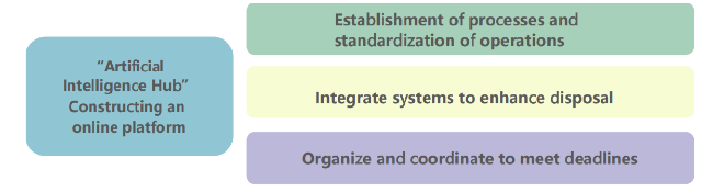
4) Construction Cost and Talent Supply Bottleneck. The integrated analysis of the Smart Community Construction and Development Drivers clusters shows that infrastructure investment and the shortage of multidisciplinary professionals are primary obstacles to community deployment (Chen et al., 2017; National Academies of Sciences et al., 2022). Future research should explore modular, open-source, hardware-software integrated solutions that leverage cloud-edge collaboration to reduce deployment costs. At the same time, it should establish industry-academia-research cooperative talent-development mechanisms, using online training platforms and community pilot projects to cultivate a scalable and replicable ecosystem of specialized professionals.
5) Beyond the widely recognized issues of privacy protection and multi-party coordination, this study—via keyword clustering and burst analysis—identifies three specific bottlenecks requiring urgent resolution: Clusters #1 (Energy Management) and #2 (IoT/AI): High-frequency data collection improves scheduling accuracy but can undermine the autonomy and energy efficiency of edge nodes. Healthcare and Governance Co-occurrence: Current participatory models struggle to meet the usability needs of elderly users. Protocol design must embed feedback loops specifically tailored to this demographic. Blockchain Intersection: Its appearance in both energy trading and privacy security themes reflects fragmented smart-contract standards across domains, creating an urgent need for unified incentive protocols to enable cross-scenario scalability.
4.3 Research hotspots and trends
Research on smart communities is continuously evolving, with emerging topics and new fields constantly developing. Consequently, researchers must acquire a comprehensive and accurate understanding of the future directions and characteristics of smart community research. Theoretically, based on the analyses and studies mentioned above, this study identified the following research characteristics and trends.
1) With the ongoing evolution of societal intelligence, the development of smart communities will increasingly integrate with artificial intelligence (AI) technology, creating a data-driven model for intelligent services and management (Ahmad et al., 2022), as illustrated in Figure 13. At the public service level, the integration of AI technology can significantly enhance the efficiency of community resource allocation. For example, by employing AI for dynamic scheduling and optimization of community resources, it can not only improve the overall operational efficiency of public services but also utilize smart voice assistants and natural language processing technologies to offer intelligent interactions and self-service options to residents. Simultaneously, through real-time sensing and data collection of information such as pedestrian and vehicle flow, energy consumption, and environmental quality within the community, and by integrating time-series forecasting, machine learning, and multi-source data fusion techniques, it becomes possible to predict and provide early warnings for water and electricity usage, public facility operations, and public health conditions. This approach offers more precise decision support for administrators. Furthermore, community management departments can implement personalized policies and services based on residents’ needs, thereby further enhancing the scientific rigor and sophistication of community governance.
Figure 13. Intelligent management model. |
2) Future research is anticipated to focus more on the expansion and innovation of blockchain technology within smart communities, while thoroughly addressing the current needs for data security and multi-party collaboration. From the standpoint of potential innovative solutions, developing a “self-regulating and energy-efficient multifunctional blockchain system” that incorporates trusted data sharing, digital identity authentication, and smart contract frameworks into community governance will lead to comprehensive data visualization of the community. This concept is highly forward-looking.
In practice, blockchain technology can be integrated into various applications, including property payments, charitable donations, and tracking volunteer service hours. By utilizing smart contracts, it can automatically execute processes such as fund distribution and reward-punishment incentives. Additionally, distributed ledger technology ensures transparency and immutability in decision-making processes. Another innovative aspect is the integration of decentralized energy trading and carbon emission management. For instance, incorporating renewable energy sources, such as distributed photovoltaic power, into the community energy network can facilitate automatic settlement and carbon credit recording, providing a robust foundation for low-carbon community development. With these modular and scalable blockchain nodes, smart communities can achieve more efficient daily governance while maintaining self-regulation and sustainable development in a constantly evolving external environment.
3) Future research is anticipated to place greater emphasis on the fundamental role of deep learning in enhancing public services and improving residents’ quality of life in smart communities through multimodal data analysis and interaction design. The utilization of complex scenario modeling and adaptive algorithms to create a “deeply perceptive community” with intelligent recognition and dynamic response capabilities is indeed feasible. For instance, video surveillance, environmental sensors (such as those measuring noise, temperature, humidity, and gas emissions), and resident behavior data can be integrated into a cohesive deep learning platform. This platform would internally fuse multi-source information to more accurately predict security risks, detect environmental anomalies, and provide personalized services tailored to the needs of diverse populations (e.g. elderly care, education, and healthcare). Additionally, personalized analysis reports can be generated based on various health monitoring metrics.
Meanwhile, optimizing the model training and inference processes can fulfill the real-time and accuracy requirements necessary for high concurrency and multimodal data processing, thereby providing effective decision support for the community (Boehm et al., 2022). By integrating these technologies and applications, the concept of a deeply perceptive community is anticipated to accelerate the advancement and evolution of smart communities in areas such as public safety management, environmental monitoring, and diverse service provision. Additionally, it will present new ideas and strategies for tackling challenges such as urban population aging and environmental changes.
4) In the coming years, the academic community is anticipated to place greater emphasis on the crucial role of smart communities in enhancing data privacy protection, Internet of Things (IoT) security, and online public opinion monitoring through innovative approaches (Cui et al., 2018; Eckhoff & Wagner, 2017). Implementing multilayered security strategies and adaptive risk management mechanisms to establish an “adaptive secure community” with compliant management and real-time protection capabilities is achievable. For instance, emerging security concepts, such as blockchain technology and zero-trust models, can be integrated into the community’s IoT system to provide distributed encryption and access control for data collection, storage, processing, and sharing. At the same time, continuous tracking and identification of potential threats can be conducted through sensor networks and monitoring systems, enabling rapid responses in the event of animals. Based on this, targeted security strategies can be tailored for various community applications (e.g. smart access control, smart homes, public sentiment monitoring), thereby reducing the risks associated with single points of failure and ensuring compliant management. By continually optimizing data encryption, access control, and security auditing measures in daily operations, the adaptive secure community will effectively address the challenges posed by cyberattacks, privacy breaches, and the spread of misinformation, offering innovative ideas and solutions for maintaining social stability and enhancing residents’ sense of security.
5 Conclusion
5.1 Conclusion of the article
Given the significance of research in the field of smart communities, an increasing number of studies on this topic have garnered widespread attention from researchers. To this end, this paper employs VOSviewer and CiteSpace for visual analysis, utilizing data sourced from the Web of Science Core Collection platform. A bibliometric analysis was conducted on research literature related to smart communities from 2000 to 2024, focusing on six dimensions: annual publication volume, journals, countries, institutions, authors, and keywords. This study provides an in-depth exploration of the development trajectory, research hotspots, and trends in the field of smart communities. The conclusions drawn from the analysis are as follows:
1) Analysis of annual publication trends revealed an exponential increase in the number of papers on smart communities between 2000 and 2024. After 2021, the field’s annual output surpassed 40 articles. Throughout this period, the disciplines of electrical and electronic engineering, computer information systems, and communications have maintained their leading roles. This study is the first to employ an exponential-fitting model to forecast quantitative growth trends in this literature, thereby offering a data-driven reference for future research planning. Furthermore, the results expose an evolutionary trajectory in which the field shifts from a predominantly technology-driven focus towards an integrated model combining technological innovation with social governance.
2) The distribution of high-impact journals and submission patterns reveals that IEEE Access, Energies, and Sustainability have the highest publication counts, whereas Applied Energy and IEEE Transactions on Smart Grid lead in citation frequency. This dual-metric analysis—incorporating both output and citation impact—offers researchers a practical guide for selecting target journals, thereby optimizing strategies for disseminating findings and planning submissions.
3) Analysis of national leadership and collaboration patterns revealed a dual-core structure centered on China (137 publications; FWCI=1.15) and the United States (68 publications; FWCI=1.22). Australia is rapidly emerging as a significant contributor, with an FWCI of 2.79. A pronounced pattern of regionalized cooperation networks is also evident. By integrating FWCI metrics with maps of international collaboration, this study elucidates the coupling mechanism between policy-driven contexts and scholarly impact. These insights provide a data-driven basis for optimizing cross-national research partnerships.
4) Analysis of core researchers and their scholarly contributions identifies Gao Weijun, Javaid Nadeem, and D.B. Smith as both highly productive and frequently cited authors. In particular, D.B. Smith’s publications garnered an average of over 130 citations. This study introduces an innovative metric that integrates each author’s H-index with their mean citation rate to pinpoint promising mentors and research teams, thereby enhancing the efficiency of academic collaboration.
5) Examination of institutional contributions and collaboration patterns shows that King Saud University and Tongji University lead in publication output. Zhejiang University, despite its modest output (n=5), exhibits high-quality dark horse characteristics, achieving an average of 158.2 citations per publication. To support emerging institutions, this study introduces a balanced quantitative indicator that integrates output and impact, guiding the development of strategies for enhancing both research quality and productivity.
6) Analysis of keywords and thematic evolution indicates that energy management, AI/IoT technologies, social governance, and privacy security are increasingly intersecting, while interest in deep learning and sustainability continues to rise. Focusing on Sustainable Cities and Communities (SDG 11), this study proposes a three-stage practical pathway: environmental sensing to support pollution reduction and optimize green infrastructure (Target SDG11.6). Participatory governance to advance inclusive urban planning and shared community services (Target SDG11.3). Regenerative technologies, such as digital twins, blockchain, and renewable-energy microgrids, enhance urban resilience and low-carbon recovery (Target SDG 11.5). Together, these elements form a toolkit that offers decision-makers and practitioners a systematic and quantifiable framework for building sustainable communities.
5.2 Innovation analysis
This study utilized advanced tools such as CiteSpace and VOSviewer to perform a comprehensive bibliometric analysis of 364 papers published between 2000 and 2024, tracking the progress of research on smart communities. The following innovations are highlighted:
1) From a knowledge perspective, a comprehensive, multidimensional, and integrated analysis of advancements in smart community research was conducted through collaboration, co-citation, and co-occurrence. This analysis offers readers extensive information to comprehend the dynamic developments within the field of smart community research.
2) From a theoretical perspective, this study developed a new knowledge framework for the field, which facilitates a clearer, more intuitive, and faster understanding of the logical structure and evolution of smart community research.
3) From a practical perspective, this study identifies current challenges and future research trends, guiding scholars in selecting appropriate research directions for their practical endeavors more effectively.
5.3 Limitation analysis
This study has some limitations that need to be highlighted. First, the research was based on raw data extracted from the Web of Science and analyzed using CiteSpace software, with a primary focus on English-language publications. Therefore, non-English literature or research conducted in other languages may have been overlooked. These limitations yield a relatively small corpus of literature, which may exaggerate the scholarly output of Europe, North America, and other English-speaking regions while understating research activity elsewhere. By excluding non-English publications—such as those in Chinese, Portuguese, and Spanish—localized case studies from Latin America, the Arab world, or within China (for example, rural smart eldercare or community microgrid pilots) are omitted. This exclusion, therefore, biases our understanding of the diversity of hot topics and regional collaboration patterns. Nevertheless, smart community research is a highly globalized, interdisciplinary field. Its core theoretical models, key technological breakthroughs, and policy frameworks are predominantly published in or widely cited by English-language literature. As a result, the identification of principal research trends and trajectories remains robust, and omitting publications in any single language does not fundamentally alter the study’s main conclusions (Joss et al., 2019). Second, this study only analyzed literature from the Web of Science database, excluding other important repositories, such as Google Scholar, ProQuest, SpringerLink, and CNKI. This selective data source may impact on the comprehensiveness of our research results. Additionally, the field of smart community research is rapidly evolving, and the analyses and predictions presented in this article are based on the current state of research, which may result in inherent limitations in terms of scope and accuracy.
To mitigate these limitations and further enhance the study, improvements can be made in the following areas:
1) Expand language coverage: Future research could involve literature searches and analyses in multiple languages to comprehensively cover the research findings across different languages.
2) Multi-Database Retrieval: In addition to the Web of Science database, other academic databases should be considered to gain a broader research perspective.
3) Dynamic Updating of Research Methods: Given the rapid development of the smart community research field, it is important to periodically reassess and update the methods and conclusions of this study to reflect the latest scientific discoveries and theoretical advancements. Adopting such a dynamic approach will better address the limitations of the current methodology and support the continued growth and rigor of research in this field.
Author contributions
Lang Zhou (Email: 20230104@wzut.edu.cn; ORCID: 0009-0002-6255-7317): Conceptualization (Equal), Formal analysis (Equal), Funding acquisition (Equal), Project administration (Equal), Resources (Equal), Software (Equal), Validation (Equal), Writing - original draft (Equal), Writing - review & editing (Equal), Data curation (Equal).
Xinting Li (Email: 202099800008@email.sdu.edu.cn; ORCID: 0009-0009-1071-5468): Conceptualization (Equal), Validation (Equal), Visualization (Equal).
Ziyi Ying (Email: 20210421@wzut.edu.cn): Conceptualization (Equal), Funding acquisition (Equal), Supervision (Equal), Validation (Equal).
Siweisi Zeng (Email: 20210451@wzut.edu.cn): Data curation (Equal), Methodology (Equal), Resources (Equal).
Jun Xia (Email: 20235155@office.dongseo.ac.kr; ORCID: 0009-0001-0936-5052): Investigation (Equal), Methodology (Equal), Software (Equal).
Data availability statement
All data generated or analyzed during this study are included in this published article.
Funding information
This research was funded by Zhejiang Province (grant number jg20220704) and Wenzhou University of Technology (grant number ky202415).
Conflict of interest
The authors declare that they have no competing interests.