


1 Introduction
Brain circulation is a global phenomenon that has far-reaching implications for science, economies, and society (Geuna, 2015; Gomez et al., 2020; Guan & Chen, 2012; Moed & Halevi, 2014; Pao, 1992; Petersen, 2018). The movement of skilled individuals across geographical borders and within regions has become increasingly prevalent in today’s interconnected world. This trend brings both challenges and opportunities for countries and organizations to increase knowledge flow while hindering brain drain worldwide (Solimano, 2006; Tarique & Schuler, 2010; Thorn & Holm-Nielsen, 2008). The policies and initiatives established by local government bodies play an essential role in promoting urban livability to attract talents. These effects include creating a favorable working environment and providing affordable living conditions. These factors are crucial for enabling employees to easily access social support networks, healthcare services, and educational facilities. For scientists who need to move between nations or within a country, these elements are particularly vital as they facilitate their mobility and re-settlement (Hu et al., 2020). Furthermore, it offers motivation to both seasoned and budding scientists to venture into uncharted territories, thereby substantially enhancing the nation’s overall scientific research standards and fostering promising advancements in individual scientific careers (Deville et al., 2014; Jin et al., 2021; Zhu et al., 2023).
For nations, it is essential to attract researchers while also preventing brain drain, as this could impede economic growth, weaken innovation, and deplete a country’s intellectual capital (Wong & Yip, 1999), especially in developing countries (Beine et al., 2001). In addressing this challenge, government policies play a crucial role in mitigating the loss of scientists. For example, China’s “Thousand Talents Plan” aims to incentivize professionals to stay or return to their home country. Furthermore, Canada’s Express Entry system and Australia’s SkillSelect program were designed to identify and invite skilled immigrants who can contribute to the country’s economy and innovation ecosystem. These initiatives provide various benefits, including research funding, career opportunities, and tax incentives, to attract and retain scholars (Cooke et al., 2014; Shi et al., 2023; Tymon Jr. et al., 2010). Favorable immigration policies, streamlined visa processes, and targeted recruitment programs can actively attract researchers (Chand & Tung, 2019). Additionally, sound education and research policies are another key strategy to curb talent outflow (Lee, 2014; Wong & Yip, 1999). A robust education system and well-established research infrastructure are crucial for retaining scientists.
Unlike the international mobility of researchers, the domestic movement of scientists allows for the exchange of knowledge, ideas, and innovation within national geographic boundaries (Florida et al., 2010; Qian, 2010). The mobility of these highly skilled individuals contributes to the creation of vibrant knowledge ecosystems and plays a crucial role in regional development, fostering economic growth, promoting an entrepreneurial spirit, and enhancing the overall knowledge base of the region ( Kalsø Hansen, 2007). This movement represents a microcosm of global researcher mobility, with its characteristics determined by domestic economic opportunities, research infrastructure, policy frameworks, and social networks in different countries. Studies indicate that regions with strong research activities, universities, and industries often attract high-skilled individuals (Mellander & Florida, 2011; Qian, 2010). The influx of these scholars not only strengthens the region’s knowledge base but also creates a positive feedback loop, as the presence of highly skilled individuals attracts further investment, employment opportunities, and collaborative networks. Conversely, regions with limited opportunities or inadequate support mechanisms may experience a brain drain of scientists, hindering regional development. To promote the mobility of researchers, regions can enhance cross-regional cooperation, establish knowledge exchange platforms, and support networks. These measures can have a positive impact on regional development (Deng et al., 2022; Ren et al., 2020). By understanding the dynamics and impacts of domestic scientists’ mobility, policymakers and researchers can formulate effective strategies, harness the potential of highly skilled individuals, and promote balanced and inclusive growth in the region.
Extensive studies have been conducted to elucidate the factors driving the movement of skilled individuals across borders and to assess the consequent impact on both host and home countries (Chepurenko, 2015; Czaika & Orazbayev, 2018; Edler et al., 2011; Yin & Zong, 2022; Yuret, 2017; Zhao et al., 2020; Zhao et al., 2019). Researchers have studied the structure and evolution of China’s high-level talent mobility network and found that talents mainly flow to core and sub-core cities (Zhang et al., 2022). Ackers (2005) pointed out that understanding the mechanism of researcher mobility is vital for formulating future policies on sustainable scientific development, which, in return, is beneficial to the development of science and technology. Petersen (2018) found that mobile researchers gain up to a 17% increase in citations relative to their non-mobile counterparts, which can be explained by the simultaneous increase in their diversity of coauthors, topics, and geographical coordination in the period immediately following migration. Liu et al. (2021) found that funding or other configurations contribute to the high performance of scientists after mobility, which is also one of the reasons that attracts scientists to migrate (Shi et al., 2023). Shi et al. (2023) also found out that the Young Thousand Talents Program in China is successful in attracting high academic caliber but not those top ones to conduct mobility and settle down in China. Cao et al. (2020) demonstrated that Chinese returnees not only produce research with greater impact and publish more frequently on an international scale compared to their domestic counterparts, but they also play a crucial role in connecting China to the global scientific network through active co-publication with researchers from their former host institutions, highlighting the significance of scientific social capital. Furthermore, Cao and Simon (2021) emphasized the significance of collaboration between academia, industry, and government to address these talent challenges and strengthen China’s position in the global innovation landscape.
However, there are few quantitative studies concerning domestic mobility patterns across institutions within a country (Ackers, 2005; Millard, 2005). This is because of the lack of high-resolution data that contain scientists’ publication records in smaller administrative divisions than the country, such as cities or states. In addition, to accurately estimate the effect of intra-country mobility on scientists, we need quantitative methods to compare groups of scientists who are similar in all academic characteristics except for the occurrence of mobility, thereby excluding the confounding effects of inherent characteristics on these metrics for scientists. In some relevant papers published by Chinese scholars, Wang et al. (2022) used the method of complex networks to analyze the flow characteristics of scientific researchers across 34 provinces in China and concluded that the flow exhibits a scale-free characteristic, where developed provinces show large inflow and outflow, while other provinces have limited mobility. Li (2021) on the other hand, conducted statistical analysis on the mobility data of scientific researchers using ORCID data, revealing the highly uneven regional distribution of mobility characteristics among Chinese researchers and a tendency for scientists to gather at Double First-Class (DFC) universities. Their research was scientifically rigorous and worthy of reference and emulation.
In this work, we tried to study domestic mobility in China, mainly focusing on two questions: What impact does mobility have on the academic performance of individuals, and what characteristics prior to their mobility determine their subsequent development in terms of local geographical constraints?
We identified 2,896 scientists who relocated from one city to another between 2014 and 2017 in China (the “moved” group) using the large-scale scientific corpus, OpenAlex. We integrated multi-dimensional scientific performance measures (Fortunato et al., 2018; Zeng et al., 2017), including productivity, citation impact, collaboration network, and level of university prestige, which is determined by whether a university is listed in the Double First-Class (DFC) Initiative in Chinese Universities (Liu et al., 2019; Peters & Besley, 2018; Wei & Zhang, 2020). DFC is an official university plan aiming to build world-class universities and includes about 140 elite universities in China. In the same period, the number of scientists without relocation in China was 89,529 in our database, so we found the contender from them as the “unmoved” group by the propensity score matching (PSM), which is commonly used in observational studies. Each “moved” scientist was paired with an “unmoved” one and this “pair” achieved a balance in which they have a similar number of publications, citations, and collaborators, as well as the level of employer universities before mobility. The effect of mobility is then estimated by the difference in academic performance posterior to mobility between the “moved” and “unmoved” groups.
We found that the “moved” scientists experienced a decrease in the number of citations and an increase in the number of collaborators after moving to a new institution compared to their “unmoved” contenders, and there was no significant change in the number of publications. In addition, there is a higher probability for scientists to switch to lower-prestige (non-DFC) universities. A further regression model revealed that the number of prior collaborators is a significant positive predictor of a scientist’s likelihood of moving to a more prestigious university; nevertheless, the number of prior publications is a negative predictor of this outcome.
This study makes a significant contribution to understanding the mobility patterns of Chinese scientists. Although the topic of scientists’ mobility has been extensively explored within countries (Ackers, 2005; Chepurenko, 2015; Liu & Hu, 2022; Millard, 2005) and across international regions (Carlson & Martin-Rovet, 1995; Thorn & Holm-Nielsen, 2008; Zhao et al., 2020), there remains a limited comprehension of its dynamics within emerging economies like China. To this end, we embarked on an investigation into the mobility of scientists encompassing various disciplines within China. Our approach to defining scientist mobility, extrapolated from publication records, was distinguished by a heightened level of rigor compared to the prevailing standards within the field.
By focusing on Chinese scientists’ mobility patterns within a country (domestic mobility), we integrated the official “Double First-Class” initiative of university classification in China in our analysis and the collaboration networks, which provides invaluable insights into how university prestige and collaboration networks influence scientists’ mobility patterns in China, further complementing existing macro-level studies that have primarily concentrated on international researcher flows or overarching movement patterns across countries (Gomez et al., 2020; Petersen, 2018; Solimano, 2006; Trippl, 2013; Verginer & Riccaboni, 2021; Yin & Zong, 2022; Yuret, 2017).
2 Literature review
2.1 Factors influencing scientists’ mobility
Scientists’ mobility is shaped by a complex interplay of personal, institutional, and systemic factors. At the individual level, researchers may relocate due to personal considerations, such as family circumstances or career ambitions(Appelt et al., 2015; Pellens, 2012). Professional factors—such as access to better research facilities, funding, or job opportunities—also play a critical role. Disciplinary cultures and publication expectations vary across fields and can influence the perceived benefits of mobility(Azoulay et al., 2017).
At the institutional and national levels, policies and incentives can significantly affect mobility decisions. For example, performance-based recruitment practices and internationalization strategies can shape how and where scientists choose to move (Hu et al., 2020; Liu & Hu, 2021). The “brain drain/brain gain” framework emphasizes how scientific mobility affects both sending and receiving countries in terms of innovation and capacity building (Jałowiecki & Gorzelak, 2004; Robertson, 2006).
Different types of mobility further complicate these dynamics. These include international moves across countries, domestic mobility within a nation, and intra-institutional transfers. Each form of movement carries unique motivations and consequences (Amelina, 2013; Chepurenko, 2015; Zweig et al., 2020). The “scientific diasporas” framework underscores the value of transnational networks formed through mobility, which facilitate knowledge diffusion across geographic and institutional boundaries (Séguin et al., 2006; Tejada Guerrero, 2012)
2.2 Effects of mobility on scientific performance
Mobility can significantly influence research productivity and impact. Moving to a new institution often provides access to improved research infrastructure, expanded collaboration networks, and diverse intellectual environments (Li & Tang, 2019; Yin & Zong, 2022). These factors may enhance academic output in the long term, although short-term disruptions are also common.
Measuring academic performance in the context of mobility remains challenging. Traditional metrics—such as publication counts, citation rates, and the h-index—may not fully capture the transitional phases in a mobile researcher’s career (Bornmann, 2014; Haunschild & Bornmann, 2023). Moreover, changes in institutional affiliation can obscure the continuity of scholarly contributions and collaborations (Jonkers & Tijssen, 2008; Petersen, 2018).
Mobility may affect not only the quantity but also the nature of the research. Shifts in co-authorship patterns and exposure to new disciplines can lead to innovative, interdisciplinary work. Conversely, temporary declines in output or recognition may occur as researchers adapt to new environments (Conchi & Michels, 2014; Waltman & van Eck, 2012).
Finally, academic performance itself can act as both a consequence and a driver of mobility. High-impact researchers are more likely to receive attractive offers, while institutions use performance indicators to evaluate and recruit talent (Costas et al., 2010; Liu & Hu, 2021). This mutual relationship creates a feedback loop between scholarly success and career movement.
3 Data and method
3.1 Scientists’ mobility data and outcome variable definition
The data used in this study were obtained from OpenAlex (Priem et al., 2022), which includes information on scientific publications worldwide and is widely used in research on the science of science (Gates & Barabási, 2023; Nishikawa-Pacher et al., 2022; Venturini et al., 2023). Given the cases of Chinese names as represented in the Pinyin and the common situations where multiple individuals share identical names, the cases where they are affiliated with the same institution, study similar topics, and cite each other’s work are rare. The OpenAlex uses a sophisticated algorithm to conduct the name disambiguation for scientists, which integrates the name strings, affiliations, citation networks, and external resources including Crossref, PubMed, ORCID, etc., and thus minimized the errors of putting scientists with identical names as one scientist.
We then defined the selection criteria for moved and unmoved scientists as follows. To investigate the impact of scientist mobility on their scientific performance and collaboration networks in China, we first selected all papers published by scientists affiliated with Chinese institutions in the OpenAlex and filtered out the “moved” scientists who conducted mobility from 2014 to 2017 in China. The migration of scientists occurs when they publish two consecutive articles at different institutions, and the year of publication of the last article in the former employer institution is regarded as the year of movement. To ensure we captured a meaningful period of work before and after the move, we required that each scientist had at least one publication both before and after the mobility year, and that their publication activity spans a multi-year window around the move (typically 2 years pre- and 2 years post-mobility, when data permitted). Scientists with multiple institutional transitions during the 2014-2017 period were excluded to isolate the effects of a single relocation. For the unmoved group, we selected scientists who remained affiliated with the same institution throughout 2014-2017. We applied the same inclusion criterion of minimum active publishing years within the window. This resulted in a total sample of 2,896 moved individuals. The “unmoved” group, which served as the contender of “moved” scientists, was made up of approximately 89,529 scientists who did not conduct mobility during this period.
To clarify our outcome measurement, we define post-mobility research performance over a standardized four-year observation window following the identified mobility event (occurring between 2014 and 2017 to ensure consistent coverage). Using OpenAlex-provided yearlypubs (yearly new publications) and yearlycits (yearly new citations), we sum the new citations for papers published during this four-year window. To avoid bias from simple productivity differences—where more papers naturally yield more citations—we normalize total new citations by the number of new publications in the same period, providing an average per-paper citation impact.
For the unmoved group, we used the same calculation method but applied a fixed observation window from 2015 to 2018 for all individuals, ensuring consistent temporal comparability. We extracted yearlypubs and yearlycits data for this period and computed the normalized average citation impact in the same manner as for the moved group. This logic applies equally to both prior and post observation periods, ensuring that all performance metrics are based on observed and validated time spans.
Importantly, to address data sparsity and variation in author career timelines, we implement a dynamic filtering approach: we include only time windows overlapping with the author’s active publishing years and adjust the measurement window length accordingly when a full four years is unavailable (e.g. for late-career movers). Cases with no overlap in the observation window were assigned zero citations and publications. This ensures that outcome measurements reflect real post-mobility activity while minimizing truncation bias or artificial inflation from unobserved years. Full details of this algorithm are provided in the SI and illustrated with an example code.
3.2 Propensity score matching (PSM)
PSM is a statistical technique widely used in observational studies to control for selection bias (Liu & Hu, 2021; Rosenbaum & Rubin, 1983). PSM is especially useful when there is no way to randomly assign subjects to different groups, such as in a non-randomized clinical trial or retrospective cohort study (Austin, 2008; Luo et al., 2010). The PSM method involves estimating the probability of each subject being assigned to a particular group, based on a set of observed covariates, and then matching subjects in the treatment and control groups who have similar scores. This helps to ensure that the groups are comparable for the observed baseline characteristics, reducing the potential for confounding. PSM can be used with both binary and continuous outcomes and has been shown to yield reliable estimates of treatment effects when implemented correctly.
The primary objective of this methodology is to reduce selection bias and improve the estimation by matching moved and unmoved groups based on their propensity scores. These scores were estimated using logistic regression or probit regression, two widely acknowledged models for estimating the likelihood of treatment assignment. The covariates X considered for propensity score estimation included research age, discipline, academic performance measurements (number of publications, citations, and collaborators in four years before the year of mobility for “moved” scientists or 2015 for “unmoved” scientists), DFC university, university prestige and geographical locations (region and part) of employer university (see Figure 1 for the list), which were selected based on their relevance to the career development of scientists and were noted as X1 to X10.
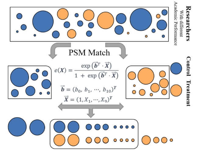
Figure 1. Visualization of PSM procedure. We collected all papers published in Chinese institutions from 2014 to 2017 to identify scientists’ mobility and selected scientists who worked in two or more institutions and whose mobility time fell between 2014 and 2017. The control group consisted of scientists with only one employer university during the observed time, resulting in a data set of about 100,000 people. Then we used PSM matching methods to find scientists with similar prior measures to the “moved” scientist and obtained 2,586 pairs of matched individuals between moved and unmoved groups. The matched pre-movement variables include (1) research age (i.e. the number of years since his/her first publication). (2) # Publications. (3) # Citation. (4) # Coauthors. (5) DFC University (i.e. the university is the Double First-Class or not) (6) University prestige (the percentile measured by the average citation per paper hosted by this university). (7) region (i.e. Beijing, Guangdong, etc.). (8) part (i.e. East China, North China, etc.). (9) discipline (i.e. Biology, Business, etc.). (10) Project 985/211 (the different Project types of the institutions, 2 for both “Project 985” and “Project 211”, 1 for only “Project 211”, and 0 for no project). The e(X) represents the estimated propensity score for a scientist with 10 covariates. Then PSM uses those scores to choose similar “moved” and “unmoved” individuals by the nearest neighbor algorithm. |
The propensity score, denoted as e(X), is calculated based on the logistic regression model for each scientist participating in the matching process. By setting the outcome variable as a binary indicator of treatment status (1 for “moved,” 0 for “unmoved”), the logistic regression model estimates the probability of each scientist receiving treatment based on the selected covariates. The propensity score signifies the likelihood of a scientist receiving treatment, considering their covariate values.
To ensure a high degree of similarity between “moved” and “unmoved” scientists after the PSM process, we employed a single nearest-neighbor approach to identify a matched “unmoved” scientist for each “moved” scientist. This procedure resulted in matched pairs with the most similar scores. Ultimately, utilizing the PSM matching method, we established 2,896 pairs of “moved” and “unmoved” scientists (See Figure 1).
3.3 Ordered logistic regression model
Ordered Logistic Regression, also known as ordered multinomial logistic regression, is a widely used statistical model for handling ordinal categorical outcomes (Fullerton, 2009; Issa & Kogan, 2014). In our study, the logit function transforms the linear combination into probabilities and is defined as:
$\operatorname{logit}\left(p_{i}\right)=\ln \left(\frac{p_{i}}{1-p_{i}}\right)=\beta_{0}+\beta_{1} \text { Publications }+\beta_{2} \text { Citations }+\beta_{3} \text { Collaborators }+\beta_{4} \text { Geo. }$
Here, pi represents the probability of observation i belonging to a specific response category, i.e. ranki =0, 1, 2. β1 to β4 are corresponding coefficients to estimate. Geo is a categorical variable controlling for geographical information, such as regional division or administrative division in China.
4 Results
4.1 Domestic scientific flow in China
The publication records of scientists, including publication time, authors, host affiliations, and topics, were collected from OpenAlex (Priem et al., 2022; Wang et al., 2019), according to which we retrieved scientists who shifted their employer universities in China from 2014 to 2017. During this period, the flow of scientists’ migration was classified by the origin and destination regions across the southern, northern, and eastern regions in China. As shown in Figure 2A, scholars in the northern region tended to relocate within the same region. Universities are not evenly distributed across regions, specifically, universities in the northern region are predominantly concentrated in Beijing, while in the southern region, they are mainly located in Guangdong and Hong Kong. As for the eastern region, major institutions are concentrated in areas like Jiangsu, Zhejiang, and Shanghai. So, most of the scientific circulations in China are among these provinces, as shown in Figure 2B.
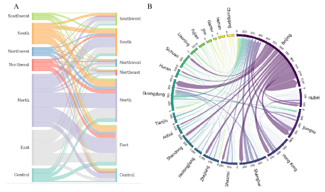
Figure 2. Chinese scientific flows at the scale of regions and provinces. A. The Sankey graph shows the scientific labor flow happening between 2014 and 2017 among regions in China (followed by Chinese administrative divisions). The left side represents the source regions, while the right side shows the destination regions. The width of a band represents the frequency of the labor flow. B. The directed circular chart shows the scientific labor flow happening between 2014 and 2017 among the main provinces in China. Only the top 20 provinces or municipalities with the highest frequency of scientists’ mobility are displayed. The width of the arc represents the frequency. |
In addition, we created scatter plots of provincial inflows vs. outflows and provincial inflows vs. the number of DFC institutions within the province. By combining Figure 3A and Figure 3B, we observed that provinces with higher inflow ratios also tend to have higher outflow volumes, indicating a proportional relationship between the inflows and outflows of scientists at the provincial level. Furthermore, in Figure 3B, it can be seen that the inflow ratios of provinces are also approximately proportional to the number of DFC universities within the province. These two scatter plots illustrate intuitively that there is a strong correlation between inflows, outflows, and the number of DFC institutions within the provinces. These findings preliminarily suggest that provinces with high inflows of scientists tend to also have high outflows. Additionally, the ratio of inflows to outflows is strongly correlated with the proportion of DFC universities within the province. Furthermore, the patterns of inflows and outflows at prestigious institutions, such as DFC, are synchronous with provincial-level inflows and outflows.
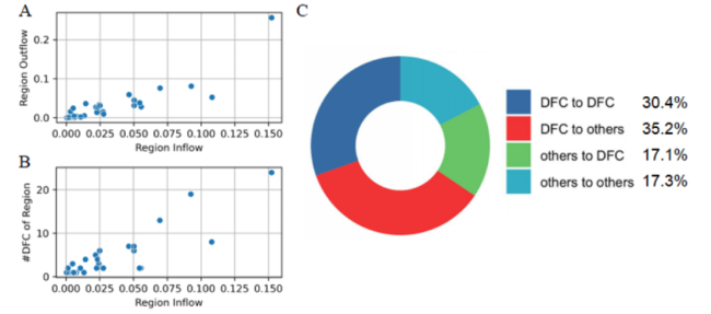
Figure 3. Chinese scientific flow in the scale of regions and university prestige. A. The scatter plot of Inflow vs. Outflow in Chinese Regions. B. The scatter plot of Inflow vs. Number of DFC institutions in Chinese Regions. C. The pie chart depicts the proportion of transitions between other institutions and DFC institutions. |
Beyond exploring the relationship between the number of provinces and DFC institutions, we also note that the prestige of institutions may influence the mobility of scientists. This inevitably raises the question: when scientists move from lower-prestige institutions to more prestigious ones, are they readily accepted?
First, based on the information we collected about DFC institutions, we aimed to highlight the actual data proportions of mobility between DFC institutions and other institutions in the flow data. As shown in Figure 3C, the data indicating movement from other institutions to DFC institutions account for approximately 50% of the total, suggesting that moving to more prestigious institutions is not an isolated occurrence within the migration data. Consequently, Section 4.7 will consider which academic factors are more closely related to scientists moving to higher prestigious institutions.
4.2 Matching contenders
We used Propensity Score Matching (PSM), a common method in observational studies (Austin, 2009; Hill & Reiter, 2006; Huang et al., 2023; Leuven & Sianesi, 2003), to find a comparative “unmoved” group of scientists who did not move, for comparison with scientists who moved between academic institutions from 2014 to 2017 in China (See Figure 1 for the schematic representation). We took several academic measurements, such as publication counts, citation counts, number of collaborators, the research starting years, and the university prestige into consideration to ensure that the “unmoved” group closely resembles the “moved” group in these key characteristics. The violin plots on the left of Figures 4A-C demonstrate the matching balance of covariate distributions between the two groups, and Figure 4D also shows the proportion of prestigious institutions that are similar before moving. The covariate balance achieved through PSM suggests that the “moved” and “unmoved” groups are now more comparable in terms of the measured covariates.
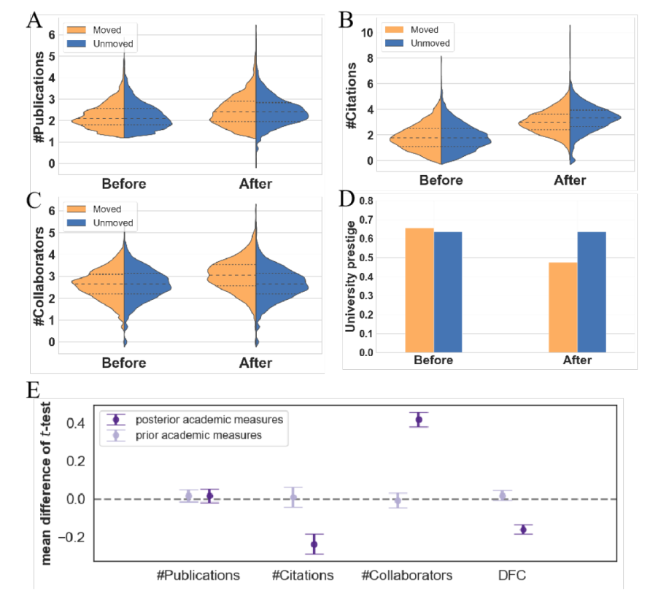
Figure 4. Comparisons of multiple measures between moved and unmoved groups of scientists. Panel A-C illustrate the distributions (in logarithmic scale) of the number of publications, number of citations, and number of collaborators, and Panel D the level of employer institution (as a percentage) for the “moved” and “unmoved” group of scientists before and after the year of mobility. Panel E displays the estimated coefficients of differences between the two experimental groups obtained using the t-test. |
4.3 Scientific collaboration and scientists’ mobility
After relocating to a new employer university, scientists did not to witness an enhancement of their productivity in the first four years after settlement (Figure 4A). However, Figure 4E indicated that “moved” scientists built up more collaborative relationships during this period, which is similar to the viewpoint proposed by Jonkers and Tijssen (2008), Kato and Ando (2017), and Liu and Hu (2022). Further confirmed in Figure 4C, after movement occurred, there was a significant difference in the distribution of the number of collaborators between the two groups. Notably, the “moved” scientists had a significantly greater number of collaborators than the “unmoved” scientists. This finding suggests that job mobility can indeed facilitate scientific collaboration by providing opportunities to expand one’s collaboration network with new colleagues.
4.4 Citation impact and scientists’ mobility
Switching to another employer university can promote collaborations by offering access to new resources and a community of scholars. However, this also brings challenges for the moved scientists, as it requires adjusting to a new scientific environment and life culture. Additionally, relocating may result in a decline in citation impact for researchers. As shown in Figure 4B and Figure 4E, the citation impact of scientists who moved and those who did not move were similar before the relocation year, with no significant difference, however, the citation impact of the “moved” scientists was lower than that of the “unmoved” scientists after moving, as reflected in the greater inconsistency of their citation impact distribution, particularly at the 25th, 50th, and 75th percentiles. Therefore, researchers should weigh the benefits and drawbacks of relocating to a new employed university and consider the potential influence on their academic prestige before making the decision.
4.5 University hierarchy of scientists’ mobility
In Figure 4D, we show the proportion of scientists belonging to the DFC universities in the two groups of scientists before and after the movement. Since the scientists in the unmoved group did not change their affiliation before and after the movement, we mainly focus on the variation of the proportion of scientists belonging to DFC universities. We noticed that the proportion of DFC universities decreased in the destination of “moved” scientists, indicating the fact that academic institutions prefer to hire faculty members who graduated from or worked in more prestigious universities. This result is consistent with previous findings that show systematic inequality and hierarchy in faculty hiring networks (Clauset et al., 2015). Similarly, in China, scholars who have been trained or have worked in top universities are often considered to possess a higher level of knowledge and expertise in their respective fields. This perception arises due to the availability of abundant resources and rigorous academic training typically offered by top-tier universities, factors that hold significant value for academic institutions (Hu et al., 2020; Kwok et al., 2011).
4.6 Heterogeneity in mobility outcomes by career stage
To further explore potential heterogeneity in mobility outcomes, we divided the scientists into two groups based on their career stage. Using the average academic age (4 years) in our dataset as the threshold, we classified researchers with no more than 4 years of academic age as early-career scientists, and those with more than 4 years as late-career scientists. For each subgroup, we conducted a series of t-tests to compare pre- and post-mobility changes in academic performance across four dimensions: number of publications, citations, collaborators, and institutional level (DFC affiliation).
Consistent with Figure 4E, both early- and late-career scientists experienced a drop in citation impact and a rise in the number of collaborators after mobility, reinforcing the general finding that mobility helps new collaborations but may disrupt citation continuity. Similarly, the proportion of scientists in DFC universities declined after mobility in both groups, echoing the institutional prestige patterns shown in Figure 4D.
However, a key difference appeared in publication output: early-career scientists showed increased productivity after moving, possibly due to better research conditions, stronger institutional support, and greater adaptability in the early stages of their careers. Mobility may also give more opportunities for younger scientists to access resources, form new collaborations, and gain visibility in broader academic networks, all of which can foster research growth. In contrast, late-career scientists showed decreased output, potentially reflecting transition costs, time-consuming adjustments, and disruptions to proven research teams and agendas.
These findings, building on the patterns in Figures 4 and 5, demonstrate that mobility’s academic consequences are not uniform but vary significantly by career stage—highlighting the need for more targeted support and incentive mechanisms, especially for senior scientists who may face higher switching costs, and for early-career researchers to maximize the benefits of their mobility.
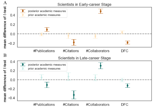
Figure 5. Comparisons between moved and unmoved groups of scientists with short and long tenure. A. The estimated t-test coefficients of differences between the two experimental groups of scientists with short tenure. B. The estimated t-test coefficients of differences between the two experimental groups of scientists with long tenure. |
4.7 Robustness check of PSM
In this section, we provide a partial elucidation of the robustness of the PSM process. First, we explained the balance of the matching process. Table 1 presents a concise statistical summary of the data before and after PSM matching. Overall, we observed that the two groups of scientists showed significant differences before matching, while disparities disappeared after matching. This shows that the enhanced balance in our matched sample bolsters the validity of our previous analyses and strengthens the reliability of the estimated treatment effects.
Table 1. Balance table of covariates before and after PSM. |
| Variable | Mean | t-Test | |||||
|---|---|---|---|---|---|---|---|
| Sample | “moved” | “unmoved” | bias% | |bias| | t | p value | |
| Research age | After PSM | 5.2289 | 5.1983 | 0.57 | 33.3 | -0.2134 | 0.8310 |
| Before PSM | 5.2289 | 5.2500 | -0.38 | 0.2090 | 0.8345 | ||
| #Publications | After PSM | 2.2392 | 2.2184 | 3.44 | 8.14 | -1.2916 | 0.1965 |
| Before PSM | 2.4497 | 2.4531 | -3.16 | -0.1912 | 0.8484 | ||
| #Citations | After PSM | 1.8512 | 1.8479 | 0.31 | 98.39 | -0.1179 | 0.9061 |
| Before PSM | 3.0165 | 3.2874 | 19.46 | -10.2247 | 0.0000 | ||
| #Collaborators | After PSM | 2.6206 | 2.6206 | -0.01 | 99.98 | 0.0030 | 0.9976 |
| Before PSM | 3.0468 | 2.6210 | -51.00 | 21.6664 | 0.0000 | ||
| DFC University | After PSM | 0.6557 | 0.6661 | -2.18 | 61.79 | 0.8186 | 0.4131 |
| Before PSM | 0.4751 | 0.6661 | 5.71 | -14.7624 | 0.0000 | ||
| University prestige | After PSM | 0.9114 | 0.9107 | 1.23 | 91.29 | -0.4624 | 0.6438 |
| Before PSM | 0.8669 | 0.9107 | 14.18 | -21.0350 | 0.0000 | ||
| Project 985/211 | After PSM | 1.1302 | 1.1520 | -2.74 | 76.10 | 1.0279 | 0.3041 |
| Before PSM | 0.6958 | 1.1520 | 11.46 | -6.0741 | 0.0000 | ||
Secondly, we considered potential endogeneity issues that may arise. Although the PSM matching process can reduce bias and the influence of confounding variables in the study, we still could not completely rule out the possibility that the transition to a new institution may impose different requirements on scientists, leading to changes in academic performance, which is the endogeneity issue we were concerned about. Therefore, more robust tests are needed. We randomly reshuffled the two groups of scientists obtained after PSM matching 100 times, re-divided them into mobile and non-mobile groups, calculated the mean differences in academic performance for each pair, and plotted the distribution. As shown in Figure 6, it is evident that except for the variable “#Publications”, the original mean differences in other academic performance variables for the two groups are not within the range of the reshuffled distribution. It explains the significant effect of changes in these variables before and after movement. To some extent, this helps to alleviate the impact of endogeneity on the experiment, indicating that mobility indeed plays a significant role in altering scientists’ academic performance.
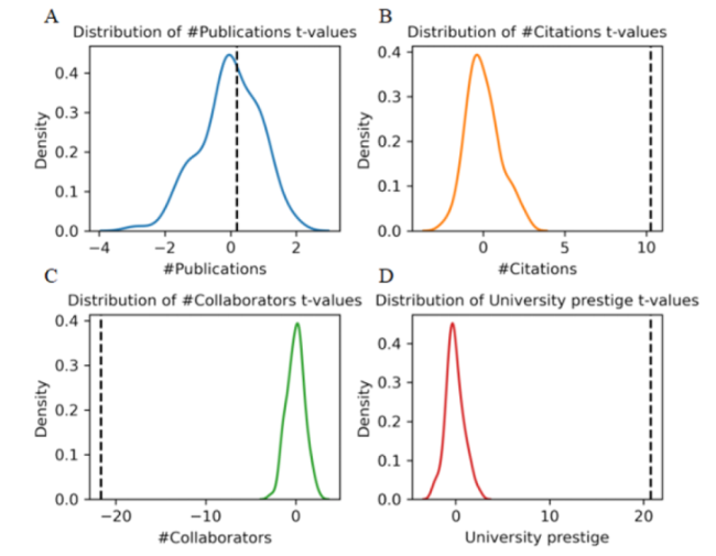
Figure 6. Distribution diagram of endogeneity test for variables. The figure displays the distribution of actual mean differences (black dashed lines) between the two groups and the mean differences generated from 100 random allocations separately. The variable names corresponding to the distribution maps A-D are consistent with those in Figure 4. |
4.8 Drivers of prestige-related mobility
The preceding analysis has revealed a decrease in the proportion of scientists moving to higher prestigious institutions after migration, which resonates with the results presented in Figure 3 of Section 4.1. Both findings indicate a certain level of resistance for scientists transitioning to higher prestigious institutions. Building on these insights, we sought to further explore the patterns of scientists moving from lower prestigious to higher prestigious institutions. Such transitions not only reflect individual career aspirations but also shed light on the distribution of resources and opportunities within the academic community.
Here we applied regression models to identify the potential factors. To achieve this, a ternary variable, rank, was employed to capture the difference in the level of the scientists’ employer universities before and after the move. This variable has three categories: a value of 2 indicates a transition from a non-DFC university to a DFC university, a value of 1 indicates the flat moves, i.e. from a non-DFC university to another non-DFC university or from a DFC university to another DFC university, and a value of 0 indicates a shift from a DFC university to a non-DFC university. Subsequently, an ordered logistic regression analysis was conducted on the outcome variable rank, considering the scientists’ pre-movement academic productivity (Model 1), citations (Model 2), and the number of collaborators (Model 3) respectively, while controlling for the geographical region in China (Regression formula is (1) in Method section). The findings are displayed in Table 2, which suggests that a higher number of citations and collaborators prior to the movement is positively associated with the likelihood of scientists transitioning to a higher prestigious university. Additionally, the scientists’ number of pre-existing publications is insignificantly related to the chance of transitioning to a higher prestigious university.
Table 2. Estimated coefficients of ordered logistic regression. |
| Model 1 | Model 2 | Model 3 | Model 4 | |
|---|---|---|---|---|
| #Publications | -0.0188 | -0.1336* | ||
| 0.0583 | 0.0664 | |||
| #Citations | 0.0755* | 0.0672 | ||
| 0.0351 | 0.0390 | |||
| #Collaborators | 0.1449** | 0.1585** | ||
| 0.0514 | 0.0580 | |||
| Region division | Yes | Yes | Yes | Yes |
| N | 2,896 | 2,896 | 2,896 | 2,896 |
| Pseudo R2 | 0.0433 | 0.0441 | 0.0446 | 0.0456 |
Note: *p<0.05, **p<0.01, ***p<0.001. |
To further examine how individual research performance relates to mobility across institutional tiers, we conducted both separate and joint estimations using ordered logistic regression models. The results, presented in Table 2, show that when the three variables—publication count, citation impact, and number of collaborators—are entered separately (Models 1-3), citation impact and collaboration intensity emerge as significant predictors of upward institutional mobility. In Model 4, where all three predictors are included simultaneously, the results remain consistent: citation impact and number of collaborators continue to show statistically significant and positive associations with mobility outcomes, while the effect of publication count becomes negative and marginally significant.
These findings corroborate the patterns illustrated in our simulation-based plots, which depict how the probability of institutional upward mobility varies with different levels of research performance (See Figure 7). The convergence between simulation and regression results highlights the central role of research quality and professional network strength in determining mobility opportunities. In particular, institutions tend to favor candidates who not only demonstrate high-impact scholarship but also maintain extensive collaborative ties, as these traits are often associated with long-term potential in research leadership, interdisciplinary engagement, and contribution to large-scale academic initiatives.
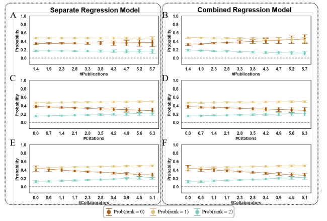
Figure 7. Estimated probabilities of institutional mobility by scientific performance indicators, based on separate and combined regression models. The x-axes represent the number of publications (A, B), citations (C, D), and collaborators (E,F). Panels A, C, and E show marginal effects from separate regression models, while Panels B, D, and F present results from a combined model including all three indicators. The y-axis indicates the predicted probability of scientists moving from a non-DFC university to a DFC one (rank = 2), making a lateral move (rank = 1), or moving from a DFC to a non-DFC university (rank = 0). |
5 Discussion
In this study, we aimed to investigate the impact of domestic scientists’ mobility on the research performance of individuals and the factors that determine their future career development. Inspired by research on cross-border mobility, we conducted a study on the intra-country mobility of scientists in China (Gomez et al., 2020; Li & Tang, 2019; Liu & Hu, 2022; Wang et al., 2015; Yuret, 2017; Zhao et al., 2020). By using higher resolution data, we classified scientific institutions according to their geographical regions, cities in China, and their prestige ranks (the DFC classification) and the PSM method to match scientists who relocated from one city to another between 2014 and 2017 with a contender group of scientists who did not move, we analyzed their academic performance before and after mobility.
Specifically, our findings reveal several interesting insights. First, the domestic mobility of scientists had a positive impact on increasing the number of collaborators. Researchers who moved between institutions within China tended to forge new partnerships, fostering a more diverse network of intellectual exchange. However, transitioning to a new institution also presents a dilemma. Despite the increased collaboration, scientists experienced a decline in their academic influence compared to the unmoved. This could be attributed to various factors, such as adapting to a different research environment, establishing new research directions, and building rapport within the new academic community.
Mediation analysis revealed that this apparent paradox stems from competing pathways: while mobility expanded collaborators (β = 0.426, p < 0.001) positively impacted research performance (β = 0.306, p < 0.001), the direct effect of mobility on citation impact remained significantly negative (β = -0.346, p < 0.001). This suggests the observed citation performance decline reflects transitional costs that outweigh the benefits of network expansion in the short term. The indirect effect (0.130) offset 38.6% of mobility’s total negative impact (-0.216), highlighting collaboration networks as a crucial buffer against relocation disadvantages. Notably, the suppression effect implies standard evaluations of mobility impacts may underestimate its true costs unless accounting for collaborative gains. This has policy implications: institutions could design transition supports (e.g. bridge funding for new collaborations) to accelerate network-mediated benefits while mitigating adaptation periods. The effects were robust across prestige tiers, though future work should examine field-specific variations in these pathways.
Furthermore, we observed a higher probability for scientists to switch to non-DFC universities indicating a preference for hiring faculty members from more prestigious institutions (Clauset et al., 2015; Kwok et al., 2011). Our regression models revealed that the number of prior collaborators was a significant positive predictor of a scientist’s likelihood of moving to a more prestigious university, while the number of prior publications was a significant negative predictor (Zhou et al., 2018). Initially adopting the DFC as a metric for assessing university reputation seemed logical, as it is a comprehensive higher education development plan launched by the Chinese government, so it could reflect the academic status and potential of a university. However, as mentioned earlier, the DFC fails to account adequately not only because it is applicable to universities in Hong Kong, but it is not as quantitative as we expected, which could lead to limitations when evaluating university prestige.
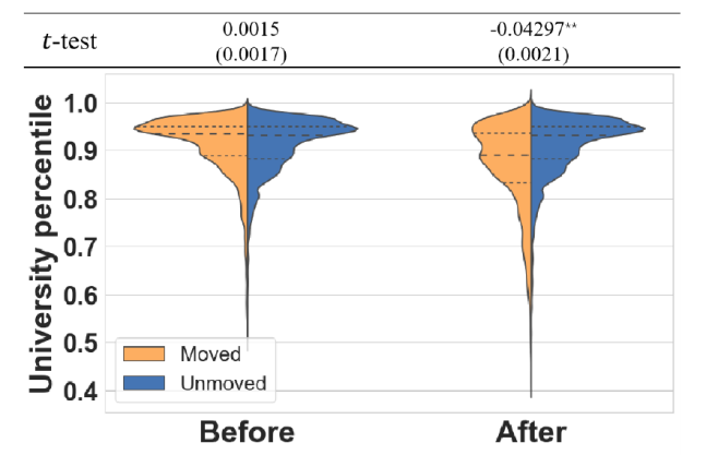
In this work, we also considered the University Percentile based on the average citations as a supplementary metric of DFC. This indicator considers a broader range of factors associated with researcher mobility and collaboration when measuring university reputation. As shown in Figure 8, the university percentile, based on the average citations per paper for scientists’ employing universities, is determined by the average citation count per paper attributed to the respective universities, with values ranging from 0 to 1. A lower value represents a lower average citation count per paper for this university, while a higher value indicates a higher average citation count per paper. The t-test results displayed at the top of Figure 8 show that there was no significant difference in the university percentiles before the year of mobility. However, a significant negative difference appears when comparing the university percentiles of moved scientists with the unmoved ones after the year of mobility. This observation means the result of University Percentile fully aligns with that of University Prestige shown in Figure 4D, confirming the consistency between these two metrics.
Figure 8. Comparison of University prestige between moved and unmoved groups of scientists. Violin plot shows the distribution of university prestige percentiles (core indicator for measuring university prestige). Statistical results are from t-tests. |
Our study contributes to understanding the multi-dimensional impact of scientists’ mobility in China, which emphasizes the importance of considering both the benefits and drawbacks of the mobility of scientists. These findings have implications for policymakers and institutions involved in scientific management and research development, as they highlight the need to create supportive environments and incentives for scientists to foster their careers while considering the potential trade-offs of mobility. These insights have valuable implications for policymakers and institutions engaged in scientific talent management and the advancement of scientific research. It underscores the necessity of establishing conducive environments and providing incentives for scientists to nurture their careers, while also carefully weighing the potential trade-offs associated with mobility. In doing so, it is essential to strike a balance that encourages mobility for professional growth while mitigating any adverse effects on research continuity and institutional stability.
Compared with previous studies on the mobility of scientific researchers in China, our work is the first to classify institutions using the “Double First-Class,” “Project 985,” and “Project 211” categories, while also integrating institutional and provincial information in the analysis. Beyond examining mobility patterns themselves, we specifically investigated how mobility affects scientists’ research output. Although our analysis relies on three widely used and readily observable indicators—publication count, citation impact, and co-authorship—we recognize that these metrics capture only a portion of the broader concept of scientific performance. Due to data limitations, especially the absence of reliable records on career progression (such as academic promotions, grant success, or administrative appointments), we were unable to include more comprehensive or qualitative measures of professional achievement. We explicitly acknowledge this limitation in our study. Future research could address this gap by incorporating alternative data sources—such as personnel files, grant databases, or survey-based career histories—to capture a wider range of mobility outcomes, including promotion trajectories, leadership roles, and project-level accomplishments.
However, it is important to acknowledge the limitations of this study. Firstly, we focused on Chinese scientists’ mobility, which might limit the generalizability of the findings to a broader population. Additionally, the data collection period from 2014 to 2017 was confined to a specific timeframe, potentially constraining our ability to capture long-term trends or changes. Moreover, our research focused solely on quantitative metrics, neglecting potential qualitative factors such as gender, nationality, and family conditions (unavailable in our database), which could provide a more comprehensive understanding of the phenomenon. While PSM aims to control selection bias, it may not eliminate it. The choice of covariates for matching and the quality of the propensity score model can influence the effectiveness of the matching process. Although we have made every effort, considering data availability, to identify covariates that might affect scientists’ academic performance and decision-making in their careers, unobserved variables that impact scientists could still lead to biased estimates, and these biases might not be easily mitigated. Another potential limitation is the data coverage for papers written in Chinese. Although the OpenAlex covers non-English papers, we’re not sure about its coverage, which may have led to an incomplete representation of scholars’ publication activities, especially in social science and humanity areas. Future research in this area could explore strategies to access and integrate data from extra sources of Chinese bibliometrics data to offer a more comprehensive understanding of scientists’ mobility in China.
In closing, the findings underscore the need for supportive policies and initiatives that balance the benefits and drawbacks of mobility, promoting collaboration and scientific progress while considering the potential trade-offs for individual scientists. Further research in this area will contribute to a deeper understanding of scientists’ mobility dynamics and its implications for scientific advancement and societal development. For example, to extend the generalizability, future studies may consider the analyses across different countries to examine intra and international scientists’ mobility. By including a diverse range of countries with varying economic, political, and cultural contexts, researchers can gain a more nuanced understanding of these factors. Moreover, investigating the phenomenon of brain gain (attraction of foreign scientists) and brain drain (loss of domestic scientists) is crucial for countries seeking to optimize their scientists’ pool (Saxenian, 2005; Zweig et al., 2008). Future research should also examine the mechanisms and factors that contribute to brain gain and brain drain, considering both the push and pull factors that influence scientists’ decisions to move across borders.
Acknowledgments
We thank OpenAlex for the scientific corpus dataset. The computation in this study was supported by the Center for Computational Science and Engineering of the Southern University of Science and Technology.
Statements and declarations
The authors have no competing interests.
Funding information
This work was supported by grants from Shenzhen Polytechnic University Research (Fund No. 6025310042 K) and the National Natural Science Foundation of China (No. NSFC62006109 and NSFC12031005).
Author contributions
Yurui Huang (Email: huangyr@szpu.edu.cn; ORCID: 0009-0001-0800-4175): Data curation (Lead), Investigation (Equal), Visualization (Lead), Writing - original draft (Lead).
Jialong Guo (Email: 11910513@mail.sustech.edu.cn): Formal analysis (Equal), Software (Lead), Writing - review & editing (Supporting).
Chaolin Tian (Email: 12131250@mail.sustech.edu.cn): Validation (Equal), Writing - review & editing (Supporting).
Shibing Xiang (Email: chibing.xiang@gmail.com): Validation (Equal), Writing - review & editing (Supporting).
Yongshen He (Email: 12132901@mail.sustech.edu.cn): Validation (Equal), Writing - review & editing (Supporting).
Yifang Ma (Email: mayf@sustech.edu.cn; ORCID: 0000-0003-0326-7993): Conceptualization (Lead), Project administration (Lead), Supervision (Lead), Writing - review & editing (Lead).
Data availability statement
All data we used in this work are publicly available, with sources from https://openalex.org.