


1 Introduction
Multi-source data fusion (MSDF) refers to the use of specific methods to process and integrate different types of information sources or relational data, thereby obtaining results that more comprehensively and objectively reflect the characteristics of the research object (Xu et al., 2017). As information sources become increasingly diverse and data types continue to expand in the era of big data, the limitations of relying on a single data source in scientific research, including limited coverage, insufficient reliability, and an inability to fully capture the complexity of research objects, have become increasingly apparent (Hong et al., 2018; Rong et al., 2019). Therefore, leveraging its ability to integrate multi-dimensional information and enhance data value, MSDF has been widely applied across various research domains (Adade et al., 2024; Liu et al., 2022; Wang et al., 2024). Among these applications, rank aggregation represents a typical and critical scenario, aiming to use appropriate methods to process ranking data from multiple sources and produce an aggregated ranking that integrates information from all aspects, thereby ensuring the reliability and objectivity of decision-making (Frank Hsu & Taksa, 2005; Lillis, 2020).
Ranking is the process of arranging a set of objects based on specific criteria to reflect their relative importance. It has been widely applied across various domains, including webpage ranking (Kayed et al., 2010), academic institution ranking (Faghri & Bergman, 2024), gene ranking (Soneson & Robinson, 2018), and sports ranking (Maanijou & Mirroshandel, 2019). With the ongoing advancement of information collection and processing technologies in modern society, the number of rankings generated based on different criteria has been steadily increasing. These rankings reflect the relative superiority and inferiority of objects from multiple perspectives. Therefore, to more comprehensively utilize information from different sources and ensure the reliability and objectivity of decision-making (Chen et al., 2018; Ossadnik et al., 2016; Ursu, 2015), appropriate methods are typically employed to process and integrate these ranking data. This process is referred to as rank aggregation (Dwork et al., 2001; Schalekamp & Zuylen, 2009; Wang et al., 2020; Zhao et al., 2019), which plays a crucial role in multiple fields, such as social choice (Caplin & Nalebuff, 1991), bioinformatics (Li et al., 2019), and recommendation systems (Pujahari & Sisodia, 2020).
Early efforts in rank aggregation sought to develop effective methods to solve the problem of inconsistent voting for political candidates in the 18 century (de Borda, 1781; de Caritat Mis, 1785). Since then, researchers in various fields have developed a wide range of rank aggregation methods for various applications to ensure more reliable results (Lin, 2010). These studies focus on the late-stage fusion phase of MSDF, with the proposed methods aiming to integrate output rankings from different data sources without involving the early processing or fusion of raw data. Among these, some studies leverage social choice theory, optimization theory, or graph theory to design algorithms specifically for handling ranking data, such as the Borda’s method (de Borda, 1781), the minimum violations ranking method (Pedings et al., 2012), and the competition graph method (Xiao et al., 2021).A few studies have also explored the application of MSDF methods to rank aggregation, such as using information fusion operators to generate the final ranking (Keyhanipour, 2025). With the substantial increase in both the quantity and types of available data, some researchers have begun exploring rank generation and aggregation methods based on heterogeneous data to further enhance the reliability of aggregated rankings. Unlike studies that focus solely on the final ranking results, these methods adopt a more comprehensive workflow, not only integrating different types of data but also considering both the relationships between the data and the internal relationships within it (Dourado et al., 2019). For example, some scholars have combined image semantic features with traditional text features for search ranking, significantly improving ranking accuracy, making it more effective compared to models that use only text (Chen et al., 2017; Lynch et al., 2016).
Although numerous rank aggregation methods have been proposed in existing studies, the effectiveness of rank aggregation depends not only on the methods employed but also heavily on the quality of the input ranking data (Deng et al., 2014; Dwork et al., 2001). In previous studies and practical applications of rank aggregation, the number and length of input rankings, as the most intuitive and computationally simple characteristics, are often considered key quantitative indicators by experts to evaluate the quality of ranking data (Tadbier & Shoufan, 2021). However, the lengths of the rankings from different sources often exhibit significant inconsistency (Li et al., 2019), thereby making it difficult to accurately assess the quality of input ranking data. Moreover, simply increasing the number of rankings does not necessarily improve data quality, as ranking data that is overly concentrated on a few objects may still lead to aggregated results lacking reliability. Therefore, when evaluating the quality of input ranking data, it is essential to consider not only the number and length of rankings but also their distribution across objects, as this distribution significantly influences the overall quality of the data.
However, existing studies often neglect to analyze the distribution characteristics of the input ranking data, which can lead to biased and misleading aggregation results. The objective of this study is to propose a simple yet effective method for measuring the quality of input ranking data based on its distribution characteristics across objects. In general, the method proposed in this study will help researchers and information managers to more accurately evaluate the quality of input data before rank aggregation, thus reducing biases and errors in the results due to poor quality input.
The remainder of this paper is organized as follows. We first introduce the concepts of information entropy, typical rank aggregation methods, and ranking correlation measurement methods in Section 2. Then, we develop two entropy-based methods to measure the quality of input ranking data in Section 3, and in Section 4, we introduce the datasets used in our experiments and how they were obtained. In Section 5, we perform an experimental analysis using several typical rank aggregation methods to demonstrate the effectiveness of the proposed measures. Finally, we conclude this study and provide an outlook for future research in Section 6.
2 Preliminaries
2.1 Information entropy
Information entropy, also known as Shannon entropy, is derived from the foundational quantitative theory of information transmission and communication (Hartley, 1928; Shannon, 1948). It measures the average amount of information contained in each symbol of an information source. Higher entropy means that the symbol probability distribution is more spread out, indicating greater randomness in the source; conversely, lower entropy implies a more concentrated probability distribution, reflecting stronger certainty in the source. Specifically, given an information source X with finite set of symbols and probability distribution P, the information entropy is defined as follows:
$H(X)=-\sum_{x \in X} P(x) \log P(x)$
Currently, information entropy has been widely applied in various research fields, such as machine learning (Wimmer et al., 2023), coding (Li et al., 2024), and data analysis (Guo et al., 2022), due to its efficiency in measuring the complexity of various objects. In particular, its application in network science, such as in quantifying the complexity of network topology, has received significant attention (Omar & Plapper, 2020). The classical network structural entropy is often defined using global graph invariants, such as node count, edge count, or degree distribution (Dehmer & Mowshowitz, 2011). These different definitions reflect the complexity and orderliness of network structure from various perspectives. Now, network structural entropy has been widely applied in numerous research fields, including financial markets (Almog & Shmueli, 2019), privacy protection (Tian et al., 2022), and identifying breakthrough topics (Xu et al., 2022).
2.2 Typical rank aggregation methods
Generally, researchers classify rank aggregation methods into two categories from the perspective of computation: optimization methods and heuristic methods (Argentini & Blanzieri, 2012). To comprehensively examine how varying distributions of input ranking information impact aggregation results of different methods, we select five typical rank aggregation methods for experimental analysis. As representatives of heuristic methods, we chose four typical methods: Borda’s method, Dowdall method, a variant of Borda’s method, and a newly proposed method called the competition graph method. As a representative of optimization methods, we select the minimum violations ranking method.
2.2.1 Borda’s method (BM)
As a classic position-based approach, Borda’s method is a conceptually simple and highly influential rank aggregation method (de Borda, 1781; Neveling & Rothe, 2021). Given m rankings R1, R2, …, Rm, for each object oj∈Ri, this method first assigns a score Bi(oj) to object oj based on the number of objects ranked below it. Then, the Borda count for object oj is the total score of m rankings, denoted as $\sum_{i=1}^{m} B_{i}\left(o_{j}\right)$. Finally, the objects are ranked in descending order of their Borda counts to produce an aggregated ranking.
2.2.2 Dowdall method (DM)
Dowdall method is another typical position-based rank aggregation method and can be regarded as a variant of the BM (Reilly, 2002). Given m rankings R1, R2, …, Rm, for each object oj∈Ri, this method first assigns a score Di(oj) to object oj, which is defined as the reciprocal of the rank assigned to it in Ri. Then, the total score for object oj is given by the sum across all m rankings, denoted as $\sum_{i=1}^{m} D_{i}\left(o_{j}\right)$. As a result, an aggregated ranking of objects can be generated by sorting the objects in descending order of their total scores.
2.2.3 A variant of Borda’s method (VB)
A variant of Borda’s method uses extension sets to manage unobserved information, specifically by accounting for the possible ranking positions of objects absent from the given rankings to address the uncertainty associated with these objects (Aledo et al., 2016). Given a partial ranking Ri, the method defines a permutation σ, which is consistent with Ri if one of the two following conditions holds for all objects os, ot ranked in Ri:
1. os and ot share the same rank in Ri,
2. If os is ranked above ot in Ri, then os must be ranked above ot in σ, and vice versa.
Moreover, σ will be said to be restricted consistent with Ri if the following two conditions hold for all objects os, ot in Ri:
1. σ is consistent with Ri,
2. ∀ok non-ranked in Ri, ok cannot be ranked between os and ot which share the same ranking position in Ri.
Therefore, the extension set of a partial ranking Ri is denoted by Er(Ri)={σ|σ is restricted consistent with Ri}.
Next, the restricted precedence extension value $V_{s t}^{r}\left(R_{i}\right)$ of Ri between os and ot is defined as follows:
$V_{s t}^{r}\left(R_{i}\right)=\frac{1}{\left|E^{r}\left(R_{i}\right)\right|} \sum_{\sigma \in E^{r}\left(R_{i}\right)} 1\left(o_{s} \text { is ranked above } o_{t}\right)$
Then, given m rankings R1, R2, …, Rm, the research define the restrict precedence extension matrix Mr=[Mst]s,t=1:n by
$M_{s t}^{r}=\frac{1}{m} \sum_{i=1}^{m} V_{s t}^{r}\left(R_{i}\right)$
Finally, Borda’s method is used to obtain a consensus ranking by sorting the column sums of Mr in ascendingorder.
2.2.4 Competition graph method (CG)
The competition graph method is an efficient approach for aggregating high-dimensional and partial rankings (Xiao et al., 2021). Given m rankings R1, R2, …, Rm with respect to n objects, this method first represents objects as nodes and employs directed weighted edges to represent pairwise comparison relationships between objects from the given rankings. Specifically, for a pair of nodes, the weight of an outgoing edge represents the number of rankings in which one node ranks above the other, while the weight of an incoming edge reflects the reverse. Based on this, the total weights of outgoing and incoming edges for each node are defined as its out-degree di+ and in-degree di-, respectively. Then, the “ratio of out- and in-degrees” (ROID) of each object is calculated as follows:
$s_{i}=\frac{d_{i}^{+}+1}{d_{i}^{-}+1}$
Finally, the objects are ranked in descending order of ROIDs to obtain an aggregated ranking.
2.2.5 Minimum violations ranking method (MVR)
As a typical optimization method, the minimum violations ranking method aims to find a consensus ranking that minimizes violations of input rankings (Ali et al., 1986; Chartier et al., 2010; Pedings et al., 2012). To solve this problem, researchers often formulate it as a binary integer linear program (BILP). Specifically, Given m rankings R1, R2, …, Rm of n objects, this method first defines the decision variable xij and the constant cij. Let
$x_{i j}=\left\{\begin{array}{lc} 1, & \text { if object } o_{i} \text { is ranked above } o_{j} \\ 0, & \text { otherwise }, \end{array}\right.$
and
$c_{i j}=\left|\left\{R_{k}: 0<r_{k i}<r_{k j}\right\}\right|-\left|\left\{R_{k}: 0<r_{k j}<r_{k i}\right\}\right|$
where Rk∈R. Note that the optimal value of the decision variable xij corresponds to the aggregated ranking, while the constants cij are related to the input rankings. Then, the MVR problem can be presented as the following BILP formulation.
$\begin{array}{c} \max \sum_{i=1}^{n} \sum_{j=1}^{n} c_{i j} x_{i j} \\ \text { s.t. }\left\{\begin{array}{c} x_{i j}+x_{j i}=1 \quad \text { for all } i \neq j \\ x_{i j}+x_{j k}+x_{k i} \leq 2 \quad \text { for all } i \neq j \neq k \end{array}\right. \\ x_{i j} \in\{0,1\} \end{array}$
Finally, a “branch and bound” algorithm based on linear programming (LP) is commonly used to solve BILP problems to obtain a minimum violation consensus ranking.
2.3 Measures of ranking correlation
The purpose of rank aggregation is to find an optimal consensus ranking that maximizes its consistency with the input rankings. There are various methods for measuring the consistency between two rankings, among which Kendall’s rank correlation coefficient (Kendall’s tau) (Kendall, 1938) and Spearman’s rank correlation coefficient (Spearman’s rho) (Spearman, 1987) are two classical and widely used metrics.
2.3.1 Kendall’s tau
Kendall’s tau measures the correlation between two rankings by evaluating the consistency of pairwise ordering. Mathematically, given two complete rankings R1 and R2 of length n, Kendall’s tau is defined as:
$\tau=\frac{2\left(N_{c}-N_{d}\right)}{n(n-1)}$
in which Nc and Nd respectively denote the number of object pairs whose orders are concordant and discordant in R1 and R2. It is obvious that the more consistent the two rankings are, the larger the value of Kendall’s tau. There are two extreme cases: τ = -1 indicates that the two lists are completely opposite, while τ = 1 signifies complete concordance.
The above definition has a flaw when dealing with rankings that include ties. Therefore, the researcher extended the Kendall’s tau to a distance metric applicable to rankings with ties in subsequent studies (Kendall, 1945). In cases where one or both rankings contain ties, Kendall’s tau-b is defined as:
$\tau_{b}=\frac{N_{c}-N_{d}}{\sqrt{\left(N_{c}+N_{d}+T_{x}\right)\left(N_{c}+N_{d}+T_{y}\right)}}$
where Tx and Ty represent the numbers of tied pairs in R1 and R2, respectively.
2.3.2 Spearman’s rho
Spearman’s rho quantifies the correlation between two rankings by assessing how consistently the ranks of each object change across the two lists. Mathematically, given two complete rankings R1 and R2 of length n, Spearman’s rho is defined as:
$\rho=1-\frac{6 \sum_{i=1}^{n}\left(r_{1 i}-r_{2 i}\right)^{2}}{n\left(n^{2}-1\right)}$
where r1i and r2i are the ranks of object oi in R1 and R2, respectively.
Spearman’s rho is a simple and intuitive measure: the larger its value, the higher the correlation between the two rankings and the stronger the ranking consistency; when the two rankings are identical, ρ reaches its maximum value of 1, and when they are completely opposite, ρ reaches its minimum value of -1.
3 Measure the quality of input ranking information
3.1 Problem statement
The rank aggregation problem is typically defined as follows: Given m rankings R1, R2, …, Rm over n objects, where each ranking represents the preferences of an individual voter, the task is to aggregate these rankings into a consensus ranking $\hat{R}$. Let Ri=(r1i, r2i, …, rin) denote the ranking provided by the voter vi, where rij is the rank of the object oj given by voter vi. In particular, rij = 0 indicates that voter vi does not rank object oj. The length of ranking Ri is therefore denoted by Li = ⌈{rij | rij > 0, 1 ≤ j ≤ n}⌉. Note that if objects ok and os are tied in Ri, we have rik = ris.
The purpose of rank aggregation is to combine rankings from multiple sources to maximize the consistency between the aggregated ranking and each input ranking, thereby obtaining a ranking that best reflects the collective preferences. Consequently, the quality of input rankings is critical in determining the quality of the aggregated ranking. Previous studies and applications often used the length and number of input rankings as quantitative indicators to evaluate their quality. However, the distribution of input ranking information across objects also directly affects the effectiveness of the aggregated ranking. To clarify this impact, two simple examples with four partial rankings over five objects are applied, which are shown in Figure 1. And we suppose that the truth ranking is a>b>c>d>e.
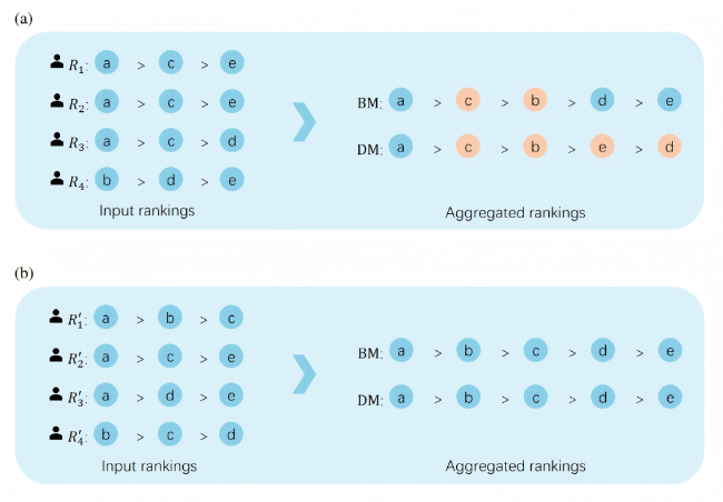
Figure 1. Comparison of rank aggregation under different distributions of input ranking information. In (a), the input information is concentrated among a few objects, whereas in (b), the input information is evenly distributed. |
We employed the BM and DM methods to aggregate these input rankings. In Figure 1(a), the distribution of input ranking information is relatively concentrated, as it not only includes two identical rankings but also three rankings that involve the comparison between objects a and c. In Figure 1(b), four distinct rankings are presented, where the recorded pairwise comparison information is evenly distributed across objects. It can be observed that when the input ranking information is evenly distributed, both methods can produce aggregated rankings that accurately reflect the true ranking. In contrast, when the distribution is uneven, neither method yields accurate aggregation results.
The above examples indicate that the even distribution of input ranking information across objects is a key factorin ensuring the accuracy of aggregation results. Therefore, developing a measure of ranking information quality based on distribution characteristics is of significant value and constitutes the core objective of this study.
3.2 Network representation of input ranking information
Each input ranking records pairwise comparison information between its objects, whereas a network represents the nodes and their interrelationships. Thus, if each object is mapped to a node in the network and the ranking information is mapped to the edges between these nodes, the network provides an effective representation of the ranking information for rank aggregation.
Specifically, we can use an undirected weighted graph G = (V, E) to represent the ranking information between objects in all input rankings. Here, V denotes the set of nodes representing the objects, and E denotes the set of edges indicating the presence of ranking information between objects. The weight of an edge between nodes vi and vj, denoted by wij, corresponds to the number of rankings that include both objects vi and vj, with 0 ≤ wij ≤ n. In particular, wij=0 indicates that no ranking contains information on vi and vj, whereas wij = n indicates that all input rankings include this information.
For example, we can transform the input ranking information from the previous example into a corresponding undirected weighted network, as shown in Figure 2. It can be observed that when the input information is concentrated on a few objects, the resulting network is relatively sparse, whereas when the input information is more evenly distributed, the network becomes denser.
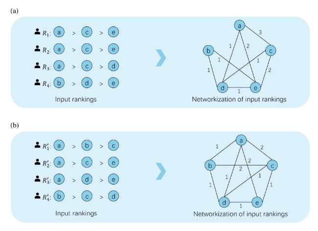
Figure 2. Network representation of input information with varying distributions. (a) illustrates the network corresponding to a concentrated input distribution, whereas (b) illustrates the network for an evenly distributed input. |
3.3 Entropy-based quality measurements of input ranking information
After transforming the ranking information into a network, we employed entropy to characterize the structural features of the network, thereby enabling a quantitative assessment of the ranking information’s quality. To explore the applicability of different types of entropy in measuring quality, we designed entropy measures across both the node and edge dimensions, capturing how information distribution influences the quality of ranking information from multiple perspectives.
3.3.1 Ranking information quality measurement based on degree entropy
For ranking data, we aimed for each object to be compared with as many other objects as possible. In the corresponding ranking network, the degree of a node reflects the number of other objects with which it has comparisons. When the degree distribution is uniform, most objects have comparisons with a similar number of other objects, indicating that the ranking information is widely covered and evenly distributed. Conversely, when the degree distribution is highly concentrated, most comparisons involve only a few objects, suggesting that the ranking information is unevenly distributed. Degree entropy can be used to quantify the uniformity of this distribution: higher degree entropy indicates a more balanced distribution of ranking information, while lower degree entropy indicates that the information is concentrated on a small subset of objects.
For a network containing N nodes, let ki denote the degree of the i-th node. Then the relative proportion of each node’s degree in the network is defined as:
$p_{i}=\frac{k_{i}}{\sum_{j=1}^{N} k_{j}} $
Building on this, the degree entropy Hd can be computed using the Shannon entropy formula:
$H_{d}=-\sum_{i=1}^{N} p_{i} \log p_{i}$
We used degree entropy to quantitatively assess the quality of the two sets of ranking data mentioned in the above section, with the results shown in Figure 3. It is clearly observed that when the overall distribution of ranking information is relatively concentrated, the coverage of comparisons among nodes is limited, resulting in lower degree entropy values. Conversely, when the ranking information is more evenly distributed, the degree entropy values are higher. This trend indicates that lower degree entropy corresponds to poorer data quality, as the information is concentrated among a few objects and cannot comprehensively reflect the relative ordering of all objects. In contrast, higher degree entropy indicates broader coverage and a more balanced distribution of information, reflecting higher data quality.
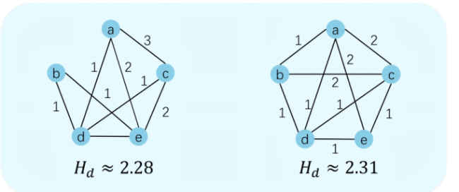
Figure 3. A measurement of input ranking information quality based on degree entropy (Hd): the more evenly the information is distributed, the higher Hd; the more concentrated the information, the lower Hd. |
3.3.2 Ranking information quality measurement based on edge-weighted entropy
The degree entropy method primarily examines the degree of network nodes to capture the global distribution characteristics of information. However, as this method fails to reflect the differences in edge weights, another approach is introduced, shifting the focus to the weights of network edges. Specifically, for an undirected weighted network derived from rankings, if the input ranking information is concentrated on a few objects, the edge weights between the corresponding nodes will be relatively large, resulting in an uneven distribution of edge weights across the network. Therefore, we can use edge weight entropy to quantify this unevenness, thereby reflecting the quality of the input ranking data.
For m input rankings, since the comparison information between any two objects oi and oj can appear at most once in each ranking, the corresponding edge weight wij takes values ranging from 0 to m. Therefore, the probability pij that a ranking contains the comparison information between oi and oj is given by:
$p_{i j}=\frac{w_{i j}}{m}$
Then, we can calculate the edge-weighted entropy based on the probability corresponding to the edge weight between each pair of nodes in the network, thereby obtaining a quantitative measure of the information distribution recorded in the m rankings. The edge-weighted entropy Hw is defined as:
$H_{w}=-\sum_{(i, j) \in E} p_{i j} \log p_{i j}$
In Figure 4, we calculated the Hw of input ranking information with different distribution characteristics based on the aforementioned example. The results similarly show that as the ranking information becomes more concentrated, the accuracy of the aggregated results decreases, and the Hw correspondingly declines, thereby reflecting lower data quality.
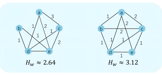
Figure 4. A measurement of input ranking information quality based on edge-weighted entropy (Hw): the more evenly the information is distributed, the higher Hw; the more concentrated the information, the lower Hw. |
4 Datasets
To investigate how the distribution characteristics of input ranking information affect the effectiveness of aggregation results and to validate the efficacy of our proposed quality measurement method, this study used both real and synthetic datasets in the following experiments. In this section, we first introduce two real datasets, and then present extensions to three commonly used ranking data generation models to enable the generation of ranking data with controllable distribution properties. All experiments were conducted on a computer equipped with an Intel Core i7-14700HX, 16 GB RAM, and an NVIDIA GeForce RTX 4070 GPU.
4.1 Real world datasets
4.1.1 Election dataset
We downloaded a dataset from the website http://www.dublincountyreturningofficer.com, containing the complete voting records of two independent elections held in Dublin, covering the northern and western areas of the Irish capital, as well as Meath County. In our experiments, we selected the voting dataset ED-00001-00000002.soi from western Dublin for empirical analysis. This dataset contains 29,988 incomplete rankings of varying lengths for nine candidates. Upon detailed examination of the original data, we found that many rankings included only a single candidate. Such rankings are essentially meaningless for ranking aggregation, as they provide no information about comparisons or outcomes between candidates. Therefore, we removed these single-item rankings. After this preprocessing, the dataset contained 28,245 candidate rankings.
4.1.2 Course evaluation dataset
We selected a course evaluation dataset from AGH University of Science and Technology in Krakow, obtained from PrefLib: A Library for Preferences, which records students’ course preferences. In this study, we used the dataset ED-00009-00000001.soc for empirical analysis. The dataset contains 146 course rankings of length 9, all of which are complete rankings. Since our experiments required incomplete rankings, we randomly removed 0 to 7 items from each ranking to create partial rankings.
4.2 Synthetic datasets
4.2.1 The Mallows model (MM)
$p_{R_{0}, \theta}\left(R_{i}\right)=\frac{1}{\phi(\theta)} e^{-\theta d\left(R_{i}, R_{0}\right)}$
where R0 and θ are the parameters of the model, representing the location and the dispersion parameters, and $\phi(\theta)=\sum_{R_{i}} e^{-\theta d\left(R_{i}, R_{0}\right)}$ is a normalization constant. Specifically, we chose the Kendall tau distance as the metric for measuring the distance between rankings.
In the Mallows model, the parameter θ (θ ≥ 0) controls the concentration of the distribution of rankings around the central ranking R0. When θ = 0, the distribution is uniform; as θ increases, the distribution becomes increasingly peaked.
To generate input ranking information with varying distribution characteristics, we introduce a distribution parameter α, which takes values in [0, ∞]. Each object is assigned an index from 1 to n, and the probability that the j-th object is selected by a voter is proportional to j-α. After generating m complete rankings, we randomly select L0 objects from each complete ranking according to this probability distribution, and reorder them according to their positions in the original ranking to construct m partial rankings. By adjusting the value of α, we can control the frequency with which each object appears in the partial rankings. Specifically, when α = 0, all objects have an equal probability of being selected, resulting in ranking information that is evenly distributed across all objects. As α increases, the probability of selecting certain objects rises significantly, leading to a more skewed distribution of the ranking data, where a few objects are ranked frequently while others appear only rarely.
4.2.2 The Plackett-Luce model (P-L)
$p_{s}\left(R_{k}\right)=\prod_{i=1}^{n} \frac{S_{o_{r_{k i}}}}{\sum_{j=1}^{n} S_{o_{k_{k i}}}}$
where $s_{o_{r_{k i}}}>0$, items with larger values of $S_{o_{r_{k i}}}$ are more likely to appear earlier in the ranking.
The consensus in this model becomes stronger as the $S_{o_{i}}$ values decrease more rapidly (Ali & Meilă, 2012). In our experiments we assign $S_{o_{i}}$ to each object using an exponential decay form defined as:
$S_{o_{i}}=S_{\max } \times r^{i-1}$
where smax is the maximum importance value, r∈(0,1) is the decay ratio.
We adopted the same approach as in the Mallows model to obtain ranking information with varying distribution characteristics. By introducing the distribution parameter α, we define the probability distribution for selecting objects by each voter. After generating m complete rankings, we randomly select L0 objects from each ranking and reorder them based on their positions in the original ranking to construct partial rankings.
4.2.3 The object inherent ability-based model (IA)
Xiao et al. (2017) proposed a ranking data generation method based on the inherent ability values of objects. The model first assume that each object oj has an inherent ability ωj, which follows a uniform distribution over [0,1]. Let R0=[r01, r02, …, r0n] be the ground truth ranking of these objects, and let rj be the true ranking position of object oj based on ωj. Intuitively, a greater ωj corresponds to a higher ranking position for oj.
Then, this model introduces the displayed inherent ability $\tilde{\omega}_{i j}$ to represent the estimate of ωj by voter vi. Since voter vi may not accurately estimate ωj of object oj for various reasons, the model assumes that $\tilde{\omega}_{i j}$ is a random variable uniformly distributed in the interval [ωj – ωj(1 – βij), ωj + (1 – ωj)(1 – βij)], where βij∈[0,1] denotes the strength of random error. A larger βij indicates voter vi ranks object oj more accurately based on ωj. Thus, a ranking Ri = [ri1, ri2, …, rin] is generated by voter vi based on the estimated values $\tilde{\omega}_{i j}$ of each object oj. In this study, we assume that all voters have the same level of estimation accuracy βij, meaning that βij = β for all i∈[1, m] and j∈[1, n]. Moreover, we assume that all rankings have the same length, that is, Li = L0∈(0, n], where i = 1,2,…, m.
Finally, we also introduce the distribution parameter α to control the distribution characteristics of the generated ranking information. Unlike the previous two models, this model allows us to generate partial rankings directly based on the specified probability distribution for selecting objects, without the need to first generate complete rankings.
5 Experimental analysis
5.1 Validation of the effectiveness of the extended data generation models
To validate the performance of the three extended models in generating ranking data with varying distribution characteristics, we generate ranking data for varying α and compute the corresponding degree entropy Hd and edge-weighted entropy Hw. Since all three models employ the same method to control the distribution characteristics of the ranking data, we use the MM model as an example for the experiments. We set n = 20, m = 1,000, and the length of rankings L0 = 2,3,4. The experimental results are shown in Figure 5. It can be observed that as the value of α increases, both entropies gradually decrease, indicating that the distribution of input ranking information among objects becomes increasingly concentrated.
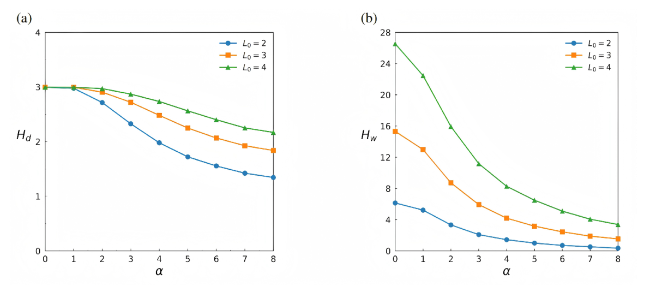
Figure 5. Degree entropy (Hd) and edge-weighted entropy (Hw) under different distribution parameters (α) with L0=2,3 and 4 respectively, where n=20, m=1,000. The results are averaged over 100 independent trials. |
5.2 Effect of distribution on ranking data quality
To examine whether an increase in the number of input rankings necessarily leads to an improvement in data quality, we generate two sets of data based on three models: baseline data and comparison data, with the numbers of input rankings denoted as mb and mc, respectively. For the baseline data, the distribution parameter α is set to 0, while for the comparison data, α is adjusted to generate ranking data with varying distribution characteristics. Then, we apply the five aggregation methods proposed in Section 2.2 to aggregate the two types of data, reflecting their quality differences through changes in the effectiveness of the aggregation results.
The effectiveness of the aggregation results is evaluated using Kendall’s tau-b between the aggregated rankings and the ground truth. The value obtained for the baseline data serves as a reference, and the relative change Δτb quantifies the difference in aggregation effectiveness between the baseline and comparison data.
The experimental results are shown in Table 1 and Figure 6, where n = 50, mb = 1,000, mc = 2,000, θ = 0.1, smax = 100, r = 0.9, β = 0.8, and L0 = 10. It can be observed that as the value of α gradually increases, the value of Δτb shows a gradual decline under all five methods. Since the comparison data contains a greater number of input rankings compared to the base data, and when the distribution of input ranking information is more uniform, the quality of the comparison data is higher, thereby improving the effectiveness of the aggregation results. However, as the distribution of ranking information becomes more concentrated, the quality of the comparison data rapidly declines, soon falling below that of the base data, thereby reducing the effectiveness of the aggregation results.
Table 1. Kendall’s tau-b between the aggregated rankings obtained by the five methods from three sets of baseline data and the ground truth rankings, where mb = 1,000, n = 50 and L0 = 10. The results are averaged over 100 independent trials. |
| Model | BM | DM | VB | MVR | CG |
|---|---|---|---|---|---|
| MM | 0.89 | 0.89 | 0.94 | 0.93 | 0.96 |
| P-L | 0.92 | 0.91 | 0.96 | 0.94 | 0.97 |
| IA | 0.93 | 0.92 | 0.95 | 0.96 | 0.98 |
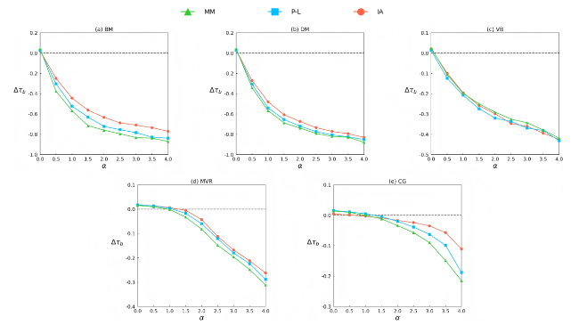
Figure 6. The relative change in Kendall’s tau-b (Δτb) under different distribution parameters (α), where n=50, mb = 1,000, mc = 2,000 and L0 = 10. Different colors represent different data generation models, e.g. green color denotes the MM. The results are averaged over 100 independent trials. |
5.3 Validation of the effectiveness of entropy-based methods in ranking data quality measurement
We conducted a series of experiments to evaluate the effectiveness of the two proposed entropy-based methods in measuring the quality of input ranking data from a distributional perspective. First, they were compared with classical ranking consistency measures to highlight the unique role of entropy-based methods in assessing ranking data quality. Then, their performance was tested on datasets of different sizes to examine their adaptability under varying conditions.
5.3.1 Comparison of entropy-based methods and classical consistency measures
To comprehensively analyze the advantages and limitations of different methods, we employed four approaches, Kendall’s tau, Spearman’s rho, degree entropy, and edge-weighted entropy, to assess the quality of data generated by three ranking data generation models with different distribution characteristics. Since the generated rankings are all incomplete, when calculating Kendall’s tau or Spearman’s rho for any pair of rankings, we consider only their common elements and finally take the average of all computed values to obtain the correlation coefficient for the dataset. The experimental results are presented in Tables 2, 3, 4, and 5, with the parameter settings as follows: n = 50, m = 1,000, θ = 0.1, smax = 100, r = 0.9, β = 0.8, and L0 = 10.
Table 2. Kendall’s tau of the data generated by the three ranking data generation models under different values of α. The results are averaged over 100 independent trials. |
| Model | α | ||||||||
|---|---|---|---|---|---|---|---|---|---|
| 0.00 | 1.00 | 2.00 | 3.00 | 4.00 | 5.00 | 6.00 | 7.00 | 8.00 | |
| MM | 0.393 | 0.394 | 0.399 | 0.439 | 0.417 | 0.383 | 0.396 | 0.347 | 0.373 |
| P-L | 0.517 | 0.540 | 0.497 | 0.564 | 0.505 | 0.519 | 0.570 | 0.551 | 0.592 |
| IA | 0.782 | 0.773 | 0.781 | 0.785 | 0.782 | 0.775 | 0.784 | 0.803 | 0.795 |
Table 3. Spearman’s rho of the data generated by the three ranking data generation models under different values of α. The results are averaged over 100 independent trials. |
| Model | α | ||||||||
|---|---|---|---|---|---|---|---|---|---|
| 0.00 | 1.00 | 2.00 | 3.00 | 4.00 | 5.00 | 6.00 | 7.00 | 8.00 | |
| MM | 0.519 | 0.510 | 0.522 | 0.532 | 0.534 | 0.462 | 0.507 | 0.535 | 0.496 |
| P-L | 0.659 | 0.661 | 0.624 | 0.685 | 0.669 | 0.638 | 0.677 | 0.660 | 0.692 |
| IA | 0.807 | 0.817 | 0.852 | 0.901 | 0.895 | 0.919 | 0.890 | 0.908 | 0.872 |
Table 4. Degree entropy of the data generated by the three ranking data generation models under different values of α. The results are averaged over 100 independent trials. |
| Model | α | ||||||||
|---|---|---|---|---|---|---|---|---|---|
| 0.00 | 1.00 | 2.00 | 3.00 | 4.00 | 5.00 | 6.00 | 7.00 | 8.00 | |
| MM | 3.912 | 3.912 | 3.895 | 3.812 | 3.688 | 3.511 | 3.351 | 3.211 | 3.102 |
| P-L | 3.912 | 3.912 | 3.895 | 3.814 | 3.688 | 3.515 | 3.354 | 3.213 | 3.113 |
| IA | 3.912 | 3.912 | 3.895 | 3.812 | 3.685 | 3.510 | 3.354 | 3.211 | 3.106 |
Table 5. Edge-weighted entropy of the data generated by the three ranking data generation models under different values of α. The results are averaged over 100 independent trials. |
| Model | α | ||||||||
|---|---|---|---|---|---|---|---|---|---|
| 0.00 | 1.00 | 2.00 | 3.00 | 4.00 | 5.00 | 6.00 | 7.00 | 8.00 | |
| MM | 7.098 | 6.400 | 5.513 | 4.964 | 4.643 | 4.444 | 4.319 | 4.232 | 4.168 |
| P-L | 7.097 | 6.399 | 5.511 | 4.965 | 4.642 | 4.446 | 4.318 | 4.232 | 4.168 |
| IA | 7.098 | 6.399 | 5.512 | 4.965 | 4.640 | 4.445 | 4.318 | 4.230 | 4.168 |
Subsequently, we aggregated the generated ranking data using five rank aggregation methods and computed the Kendall’s tau-b between the aggregated rankings and the ground-truth rankings, with the results shown in Figure 7. It can be seen that as α increases, the consistency between the aggregated results and the ground-truth rankings for the data generated by the three ranking data generation models under the five aggregation methods gradually decreases, indicating that data quality declines as the input ranking information becomes more unevenly distributed among the objects. Therefore, the effectiveness of the four data quality measures can be evaluated by examining their measurement results on the data under different values of α.
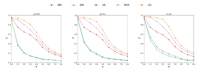
Figure 7. The Kendall’s tau-b (τb) under different distribution parameters (α), where n = 50, m = 1,000, and L0 = 10. The results are averaged over 100 independent trials. |
For the two classical ranking consistency measures, Tables 2 and 3 show that their results fluctuate non-monotonically as α increases, indicating that these methods cannot effectively capture the changes in data quality caused by variations in the distribution characteristics of the ranking data. For degree entropy, as shown in Table 4, when α increases slightly, its value changes little; as α increases further and the unevenness of the data distribution becomes more pronounced, the degree entropy decreases steadily, indicating that it can reflect the quality differences caused by variations in the distribution characteristics of the ranking data, particularly when the data distribution is highly uneven. Finally, as shown in Table 5, edge-weighted entropy decreases gradually as α increases; compared to degree entropy, it is more sensitive to changes in α and can more effectively reflect the quality differences caused by variations in the distribution characteristics of the ranking data.
5.3.2 Performance of entropy-based ranking data quality measures across different data scales
We further conducted experiments to evaluate the performance of the two entropy-based methods on datasets of different scales. Specifically, using three data generation models, we generated varying numbers of rankings under four conditions m = 50, m = 500, m = 5,000 and m = 50,000. The quality of each dataset was then assessed using degree entropy and edge-weighted entropy. The experimental results are shown in Figure 8 and Figure 9, where n=50, θ=0.1, smax = 100, r = 0.9, β = 0.8, and L0 = 10.
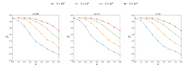
Figure 8. Degree entropy (Hd) under different distribution parameters (α) and numbers of rankings (m), where n = 50 and L0 = 10. The results are averaged over 100 independent trials. |
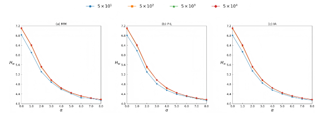
Figure 9. Edge-weighted entropy (Hw) under different distribution parameters (α) and numbers of rankings (m), where n=50 and L0=10. The results are averaged over 100 independent trials. |
As shown in Figure 8, for degree entropy, when the dataset is relatively small (i.e. m=50), degree entropy gradually decreases as α increases. However, as the dataset size grows, the change of degree entropy with increasing α initially remains stable and then gradually declines, and the initial stable phase becomes more pronounced with larger dataset sizes. This indicates that when the dataset is large and the unevenness of the data distribution is relatively low, degree entropy has limited capability to effectively measure data quality.
For edge-weighted entropy, as shown in Figure 9, it exhibits a decreasing trend with increasing α across datasets of all sizes. This indicates that edge-weighted entropy can effectively capture variations in data distribution, and its applicability is broader than that of degree entropy regardless of dataset size.
5.4 Analyzing the computational efficiency of entropy-based methods
To analyze the computational efficiency of degree entropy and edge-weighted entropy under large-scale ranking data, we use ranking data generation models to generate datasets with varying values of n and m. We then measure the time required by these two entropy-based quality metrics to process the generated datasets. Since this experiment primarily depends on the size of the dataset rather than the specific data generation model, we generate the required data using only the IA. The experimental results are shown in Figure 10 and Figure 11, where L0 = 0.1×n, θ = 0.1, smax = 100, r = 0.9, α = 0.2 and β = 0.8.
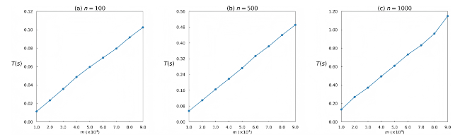
Figure 10. Computational efficiency of degree entropy (Hd) under different numbers of objects (n) and rankings (m). The results are averaged over 100 independent trials. |
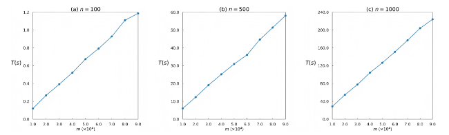
Figure 11. Computational efficiency of edge-weighted entropy (Hw) under different numbers of objects (n) and rankings (m). The results are averaged over 100 independent trials. |
As shown in Figure 10 and Figure 11, when the number of ranking objects reaches 1,000 and the number of rankings reaches 9×10⁴, both entropy-based methods can complete the computations within a short time, indicating that they maintain high computational efficiency in large-scale ranking scenarios. Among them, degree entropy performs better than edge-weighted entropy. In addition, when n is fixed, the computational time of both methods increases approximately linearly with m, further demonstrating that they can remain efficient even when processing a larger number of rankings.
5.5 Collaborative analysis of the length and distribution of input rankings
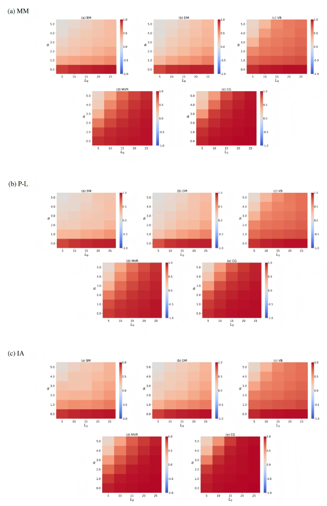
Furthermore, we also examined the combined impact of the length and distribution of input rankings generated by the three models on aggregation effectiveness. The experimental results are presented in Figure 12, with n = 50, m = 1,000, θ = 0.1, smax = 100, r = 0.9, and β = 0.8. Each heatmap cell shows the Kendall’s tau-b for a specific combination of parameters L0 and α. In the heatmaps, the color gradient of the cells from blue to red indicates a gradual improvement in the effectiveness of the aggregation results.
Figure 12. The collaborative impact of the length of input rankings (L0) and distribution parameters (α). Each cell represents Kendall’s tau-b under different combinations of L0 and α. The gradual change in color from blue to red indicates a gradual increase in Kendall’s tau-b. The results are averaged over 100 independent trials. |
For the data generated by the three models, it can be observed that as the value of α increases, an increase in the input ranking length L0 causes the red cells to gradually deepen. This indicates that increasing the ranking length L0 can mitigate the decline in aggregation effectiveness caused by the unequal probability of each object being selected for ranking. In particular, the MVR and CG methods outperform the other three methods in significantly improving aggregation effectiveness as the ranking length L0 increases. This is because both methods leverage pairwise comparison information between objects. As the ranking length L0 increases, more node pairs become connected in the network. Even if these edges have low weights, MVR and CG can still effectively utilize the available comparison information to enhance aggregation performance.
5.6 Empirical analysis of entropy-based ranking data quality measurement methods
We validated the effectiveness of degree entropy (Hd) and edge-weighted entropy (HW) in assessing ranking data quality from a distributional perspective using two empirical datasets. First, we computed the initial Hd and HW for both datasets: for the election dataset, Hd = 2.192 and HW = 3.570; for the course evaluation dataset, Hd = 2.196 and HW = 3.581. Then, to construct datasets with varying distribution characteristics, we randomly selected a ranking with a certain number of occurrences from each dataset, increased its occurrences while reducing those of other rankings to keep the total number of rankings constant, and recalculated the corresponding Hd and HW at each step. The experimental results, shown in Tables 6 and 7, illustrate the trends of Hd and 𝐻W as the occurrences of the selected ranking change in the two datasets. Here, mn represents the increased number of occurrences of the selected ranking in the dataset.
Table 6. Degree entropy (Hd) and edge-weighted (HW) of the election dataset under different distribution characteristics, with n=9 and m=28,245. The results are averaged over 100 independent trials. |
| Method | mn | |||||||
|---|---|---|---|---|---|---|---|---|
| 1,000 | 2,000 | 3,000 | 4,000 | 5,000 | 6,000 | 7,000 | 8,000 | |
| Hd | 2.191 | 2.188 | 2.183 | 2.178 | 2.171 | 2.156 | 2.118 | 2.082 |
| HW | 3.568 | 3.561 | 3.548 | 3.536 | 3.516 | 3.478 | 3.383 | 3.292 |
Table 7. Degree entropy (Hd) and edge-weighted (HW) of the course evaluation dataset under different distribution characteristics, with n=9 and m=146. The results are averaged over 100 independent trials. |
| Method | mn | |||||||
|---|---|---|---|---|---|---|---|---|
| 15 | 30 | 45 | 60 | 75 | 90 | 105 | 120 | |
| Hd | 2.195 | 2.191 | 2.189 | 2.181 | 2.177 | 2.173 | 2.166 | 2.158 |
| HW | 3.577 | 3.566 | 3.558 | 3.539 | 3.527 | 3.517 | 3.496 | 3.473 |
Based on Tables 6 and 7, as the value of mn increases—indicating that the information distribution in both datasets becomes increasingly uneven—both Hd and HW exhibit a decreasing trend. This indicates that, for these two real-world datasets from different domains, both entropy-based methods can effectively capture changes in data quality as the distribution characteristics vary.
6 Conclusion and discussion
Rank aggregation plays a crucial role in various academic studies and practical applications, and the quality of input rankings significantly affects the effectiveness of the aggregation results. In this study, we propose two general and intuitive methods for measuring the quality of ranking data from a distributional perspective. Specifically, we first convert the input rankings into an undirected weighted network and then use degree entropy and edge-weighted entropy, two types of network structural entropy, to quantify the quality of the ranking data. We then validate the effectiveness and applicability of the proposed methods through experiments on both real-world and synthetic datasets. The results of numerical experiments indicate that an increase in the number of input rankings does not necessarily lead to improved data quality, as the distribution characteristics of the ranking information also play a critical role in determining quality. We further confirm that, compared with traditional consistency measures, the two entropy-based methods can more effectively assess the quality of input ranking information from the perspective of information distribution and demonstrate good computational efficiency on large-scale datasets. Moreover, different rank aggregation methods show varying performance when handling unevenly distributed rankings. Increasing the length of input rankings can enhance aggregation effectiveness, particularly for methods that fully utilize pairwise comparison information between objects, where this effect is more pronounced.
It should be noted that the quality of ranking data is influenced by multiple factors. This study primarily focuses on the impact of the distribution characteristics of ranking data on its quality. Future research should further investigate other potential influencing factors, such as the effect of conflicts present in the data on ranking quality.
Acknowledgment
We would like to thank the anonymous reviewers for their valuable comments and suggestions.
Funding information
This work was financially supported by the National Natural Science Foundation of China (Nos. 72571031, 72401032, 72201035), the Innovation Teams Project in Ordinary Universities of Guangdong Province (No. 2024KCXTD050) and the Guangdong Basic and Applied Basic Research Foundation (No. 2025A1515011586).
Author contributions
Yishan Liu (202421250036@mail.bnu.edu.cn): Conceptualization (Equal), Methodology (Equal), Data curation (Lead), Formal analysis (Equal), Software (Lead), Writing - original draft (Lead), Writing - review & editing (Equal).
Yu Xiao (xiaoyu23@bnu.edu.cn, ORCID: 0009-0008-0744-3097): Conceptualization (Equal), Formal analysis (Equal), Methodology (Equal), Funding acquisition (Equal), Project administration (Equal), Writing - review & editing (Equal).
Xin Long (longxin14@nudt.edu.cn): Conceptualization (Equal), Formal analysis (Equal), Investigation (Equal), Writing - review & editing (Equal).
Jun Wu (junwu@bnu.edu.cn): Conceptualization (Equal), Formal analysis (Equal), Methodology (Equal), Funding acquisition (Equal), Project administration (Lead), Writing - review & editing (Equal).
Data availability statements
The data that support the findings of this study are available on request from the first author.